
Annotate Tab
Under the "Annotate" step you have the option of performing manual curation. While manual curation is not required, we suggest at least looking at several gene models and the output from the tools along with provided evidence to see if the gene models are most likely accurate. The manual curation function in GenSAS is performed using an integrated Apollo instance. Apollo not only provides manual curation functionality, but also tracks all changes made and which user made them on the "Apollo" tab, which is useful for collaborative annotation projects. To learn how to share your GenSAS project, please see the "Sharing Projects" section of the User's Guide.
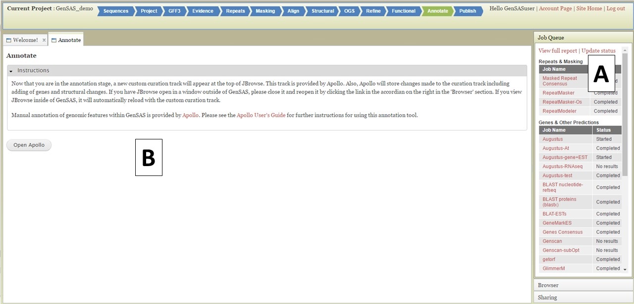
Figure 44. Annotate tab in GenSAS.
Under the "Annotate" tab, you will see a "Open Apollo" button (Fig. 44B). You can either open Apollo using that button, or open Apollo through the "Browser" section of the Job Queue (Fig. 44A). Please see the "Apollo and JBrowse" section on details on how to open Apollo/JBrowse. In the "Apollo" tab, there is a JBrowse interface on the left and you will now see a "User-created Annotations" track at the top (Fig. 45A). This is where any manual annotation changes will be entered. The changes made to the "User-created Annotations" track are logged on the Apollo interface on the right, under the "Annotations" tab (Fig. 45B). To control which data tracks are visible in JBrowse, click on the "Tracks" tab in the Apollo interface (Fig. 46A). Expandable sections appear for each data track type. Expand the section and toggle the tracks on and off. If you would like to use the normal JBrowse Track Selector, you can also toggle that on and off in the Apollo interface (Fig. 46B).
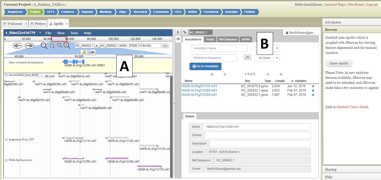
Figure 45. User-created Annotations track in JBrowse.
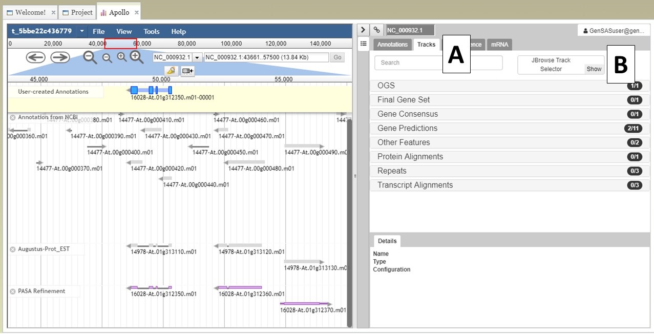
Figure 46. Turning tracks on and off in JBrowse window.
For detailed instructions on Apollo, and some information on manual curation, we recommend the Apollo User's Guide. Another good resource is "Annotation for Amateurs" which has tutorials on annotation. Per the Apollo manual, the major steps of manual curation are:
- Locate a region of the chromosome that you want to annotate in the JBrowse tab and look for gene models that might need manual curation.
- Look at the job and evidence tracks and decide if there is a likely gene model to use as a starting point.
- Drag the putative gene model to the "User-created Annotations" track to use as the initial gene model.
- Edit the gene model structure (UTRs, intron/exon junctions, start/stop codons) if necessary.
- Check the edited gene model against existing homologs by exporting the sequence and searching a protein database.
- Assign functional assignments using the Gene Ontology (GO) database and add the information to the feature notes.
Not all gene models will need editing, but some gene models will benefit from manual curation. In the GenSAS User's Guide we will only cover the basics of using Apollo and provide some examples of manual curation (see example below). To move a gene model to the "User-created Annotations" track, double click on the model until it is highlighted with red borders (Fig. 47A) and then click and drag the model to the "User-created Annotations" track (Fig. 47B). Also note that when a gene model is selected, common intron/exon junctions across all datasets are also indicated with red borders (Fig. 47C).
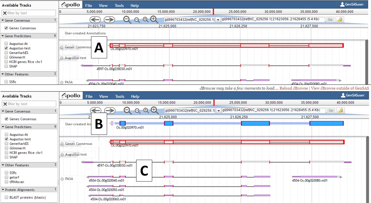
Figure 47. Dragging gene model to User-created Annotations track.
Once the gene model of interest is in the curation track, you can zoom in to the base level quickly by right-clicking on the model and selecting the "Zoom to base level" option (Fig. 48). This is useful for looking at intron/exon junctions and start/stop codons. You can also download the nucleotide or protein sequence of the gene model by right-clicking on the gene model and selecting the "Get sequence" option (Fig. 49). This is useful for getting the protein sequence for searches against a protein database during the manual curation process.
.jpg)
Figure 48. Zooming to base level of gene model.
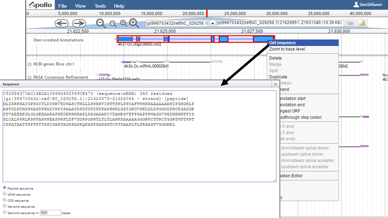
Figure 49. Obtaining sequence of gene model.
Here is an example of a manual curation of a gene model in chromosome 1 of rice. In Figure 50, you will see the JBrowse window at the "Annotate" step. The data tracks are marked to help describe the data that will be used:
- "NCBI annotation" is the imported GFF3 data of the annotation that is available in NCBI for the sequence (chromosome 1 of rice).
- "Refined Consensus" is a genes consensus that was created in GenSAS at the "OGS" step and was then refined with rice ESTs (from NCBI, uploaded by user) during the "Refine" step.
- "Augustus-RNA-seq trained" is the results of a trained Augustus job using the BAM file from the TopHat alignment of RNA-seq reads to the sequence being annotated.
- "PASA, rice ESTs" is a PASA job from the "Align" step that used rice ESTs that were uploaded by the user.
- "TopHat, rice RNA-seq" shows the results of the TopHat alignment of the user-uploaded RNA-seq reads to the sequence being annotated.
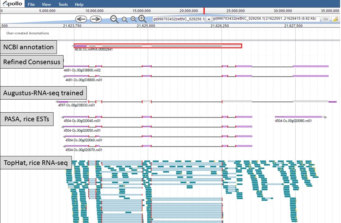
Figure 50. Manual curation example. See track descriptions above figure in text.
You can see that when the NCBI gene model is selected (Fig. 50), that the common intron/exon junctions are marked across all datasets in JBrowse. Also notice that there are differences between the annotation from NCBI and the alignments and gene predictions job results based on transcript evidence. This looks like a good candidate for manual curation. For this example, let's move the gene models we want to compare to the "User-created Annotations" track. Based on the RNA-seq data, let's look at a gene model from the "Refined Consensus" track (Fig. 51A), "PASA, rice ESTs" track (Fig. 51B), and the "NCBI annotation" track (Fig. 51C). Figure 51 is marked to show which gene model in the "User-created Annotations" track corresponds to which gene model in the evidence tracks.
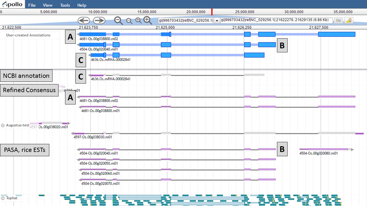
Figure 51. Three gene-models moved to User-created Annotations track.
Since there is RNA-seq evidence for this project, let's compare each of these gene models to the RNA-seq data (you can use EST evidence alignments if you don't have RNA-seq data). In Figure 52, the gene models from the "NCBI annotation" and "PASA, rice ESTs" are selected and show that most of the intron/exon junctions in these gene models are supported by the evidence in the other tracks (see red marks at junctions within black boxes). When the gene model from the "Refined Consensus" is selected (Fig. 53), most of the intron/exon junctions are not supported by the evidence except for a few (see inside black box).
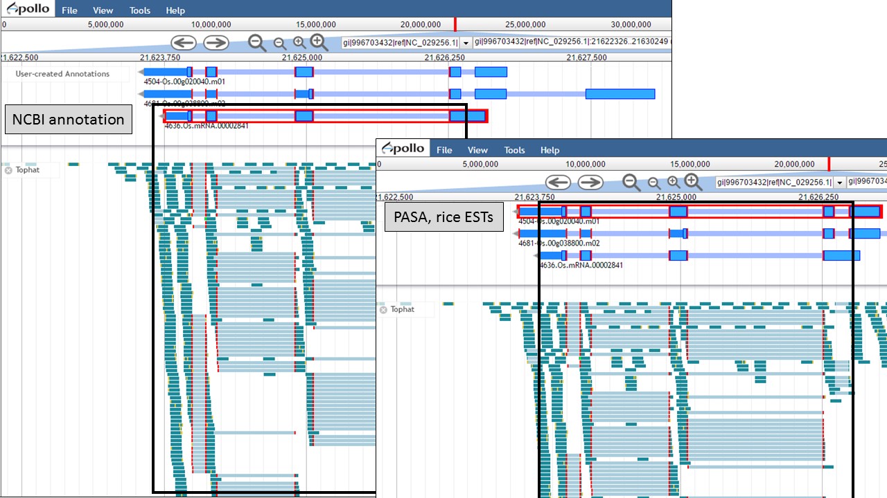
Figure 52. Intron/exon junctions in NCBI and PASA based gene models are supported by other data.
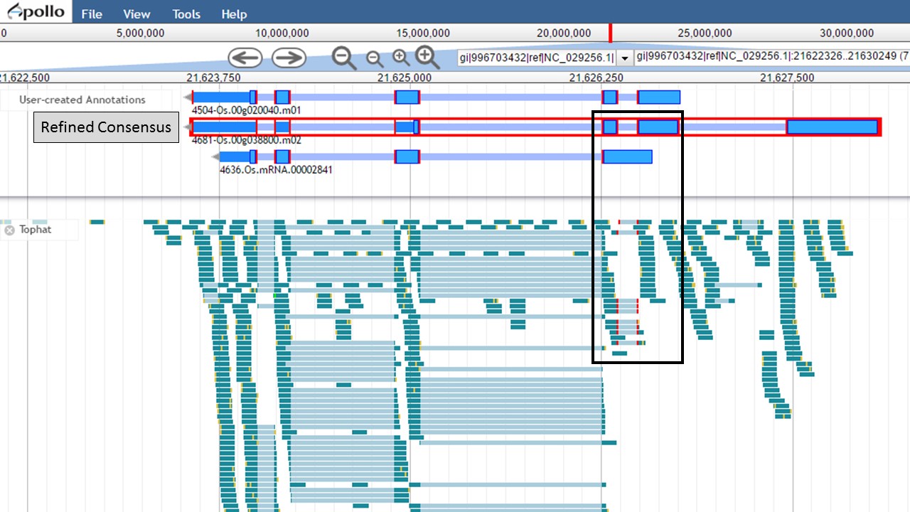
Figure 53. Few intron/exon junctions in Refined Consensus gene model are supported by other data.
Since the "Refined Consensus" gene model is not very well supported by transcript data, let's delete it from the "User-created Annotations" track. Select the gene model by double-clicking on it, then right-click with the mouse and select the "Delete" option (Fig. 54).
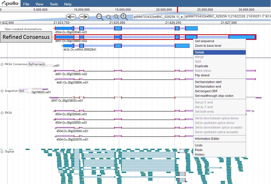
Figure 54. Deleting a track from the User-created Annotations track.
Now there are two gene models left, the "NCBI annotation" and the "PASA, rice ESTs" models (Fig. 55). The two gene models have different start positions and both lack 5' UTRs.
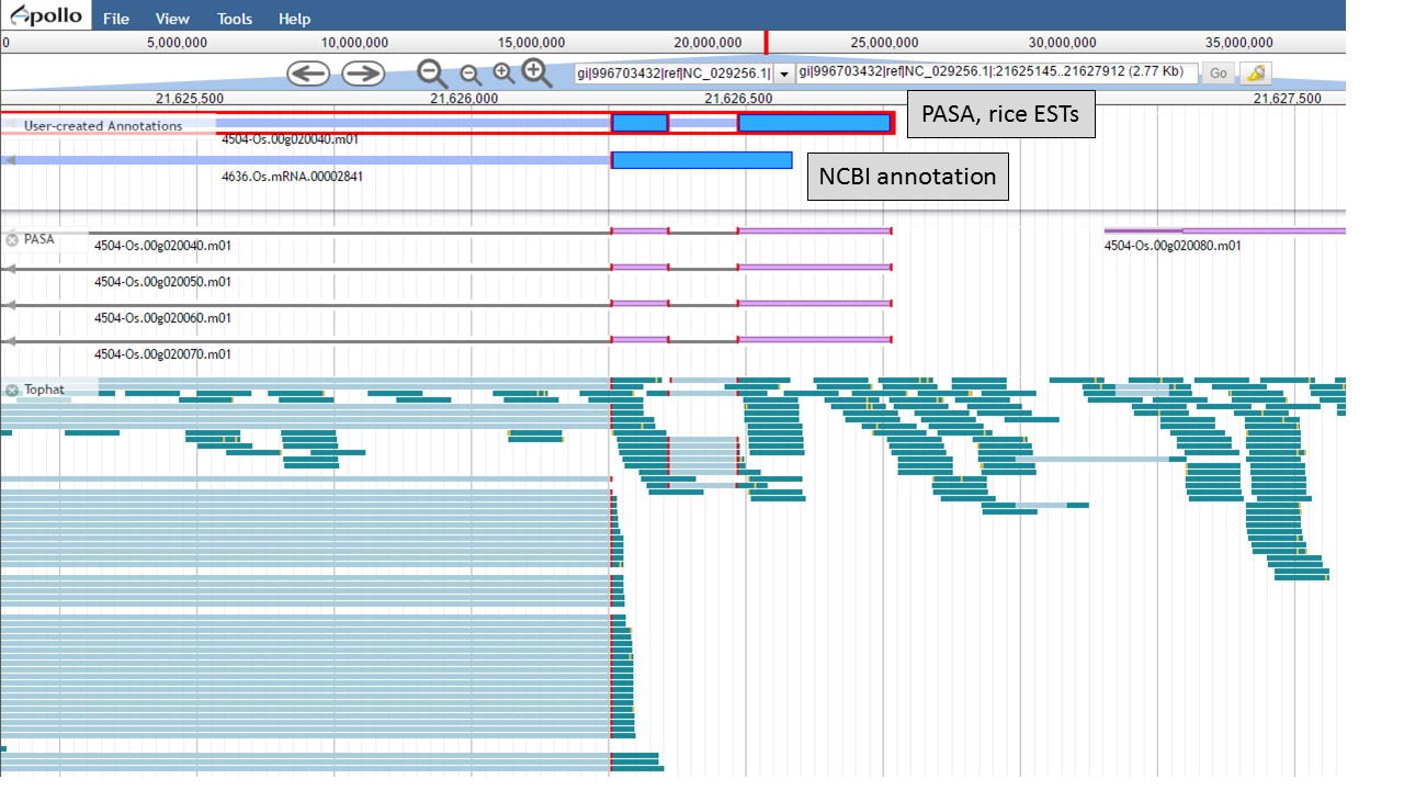
Figure 55. Two remaing gene models, with different start positions.
Let's look at the start codon for each model. When we zoom in to the base level (see Fig. 48 above for directions), we see that the start codon for the NCBI annotation is "ATG" and the start codon for the PASA gene model is "AAG" (Fig. 56). Since the PASA gene model is based on alignments with ESTs, the gene model structure was based on matches with EST evidence. This means that the location of the start on the PASA gene model is more likely the start of the 5' UTR.
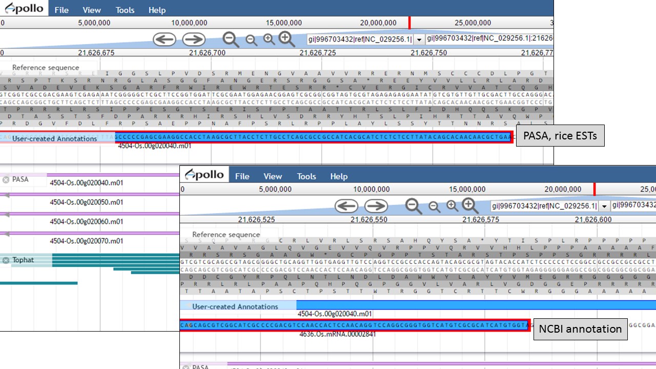
Figure 56. Start codon sequences on both gene models.
To set the translation start on the "PASA, rice ESTs" gene model, use the "NCBI annotation" start codon location as a guide to find the start codon. Once the start codon of "ATG" is located on the "PASA, rice ESTs" sequence, place the cursor at the beginning of the codon, right-click and select the "Set translation start" option (Fig. 57).
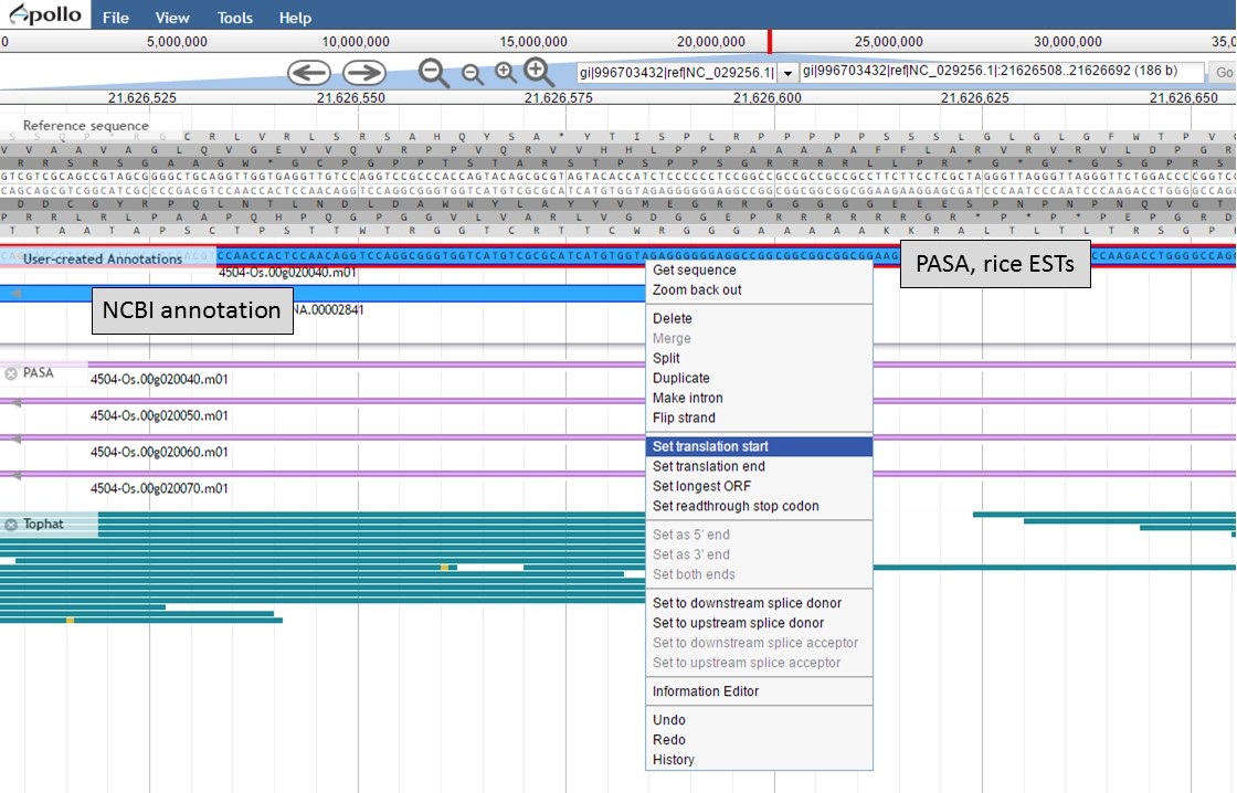
Figure 57. Setting translation start on "PASA, rice ESTs" gene model.
Both gene models now have the same start codon, but the "PASA, rice ESTs" model also has the 5' UTR region (Fig. 58).
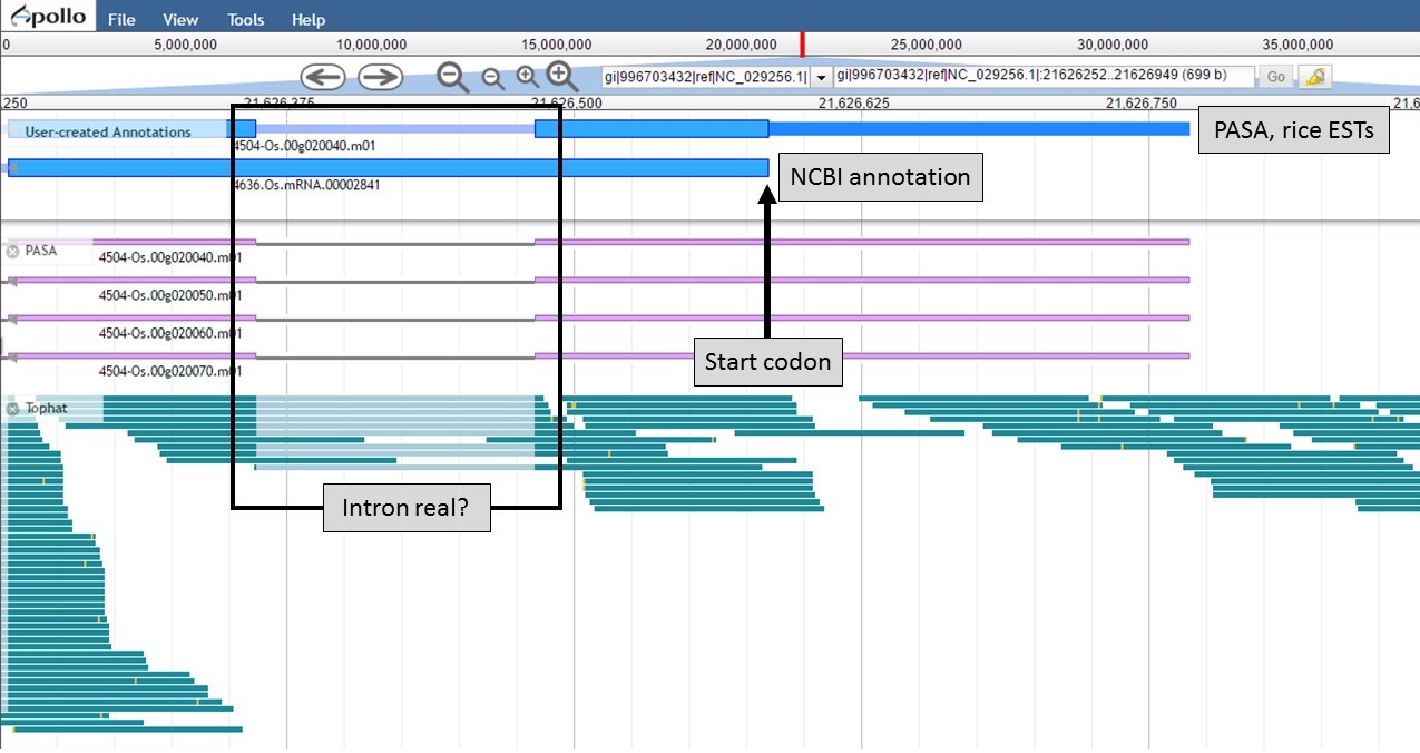
Figure 58. New 5' end of gene models and closer look at intron region.
At the 3' end of the gene model, the stop codons are in the same location, but the transcript evidence is supporting a longer 3' UTR region in the "PASA, rice ESTs" model (Fig. 59). Based on the evidence, the 3' UTR of the "PASA, rice ESTs" is probably more accurate.
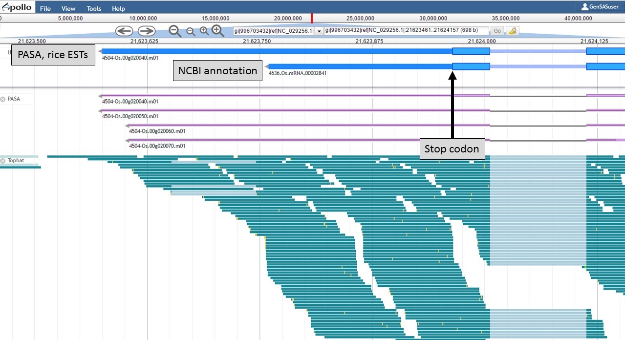
Figure 59. 3' end of gene models.
Now that the ends of the gene models have been examined, we need to determine if the first intron in the "PASA, rice ESTs" gene model is real or not. In Figure 58, a box around the intron area shows that there is EST and RNA-seq evidence support for the intron in the "PASA, rice ESTs" model. Let's look closer at the proteins coded by these gene models. Using the "Get sequence" function for each gene model (see Fig. 49 above for directions), we see that each gene model produces a different length protein (Fig. 60). The "NCBI annotation" gene model only encodes for a protein of 60 amino acids long while the "PASA, rice ESTs" gene model produces a protein of 176 amino acids. If we look closer at the "NCBI annotation" gene model, there is a stop codon in the gene model after 60 amino acids. The stop codon in the "NCBI annotation" model also sits within the intron of the "PASA, rice ESTs" gene model that is missing from the "NCBI annotation" (Fig. 58). If you look at the protein sequence alignment in Figure 60, the amino acids that are in bold correspond the first exon of the "PASA, rice ESTs" gene model. The exon-intron splice site sequences can also be examined. The common eukaryotic splice junction has a structure of 5'-exon]GT/AG[exon-3'. If the splice site is non-canonical, Apollo marks it with a orange exclamation mark so the annotator will take a closer look.
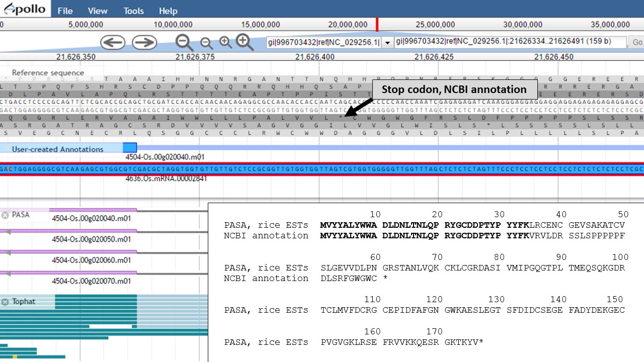
Figure 60. Proteins from each gene model and the location of the stop codon in the NCBI annotation model.
But which protein is more likely? Let's use NCBI protein BLAST to see if there are any related proteins. You can also use SmartBLAST which compares the closest protein matches graphically (Fig. 61). The protein encoded by the "PASA, rice ESTs" model has a DUF866 domain and is similar to other proteins of unknown function. The protein from the "NCBI annotation" is a truncated version of the same unknown protein. This indicates that the "PASA, rice ESTs" gene model that we edited is not only supported by the EST and RNA-seq evidence, but also by protein similarity.
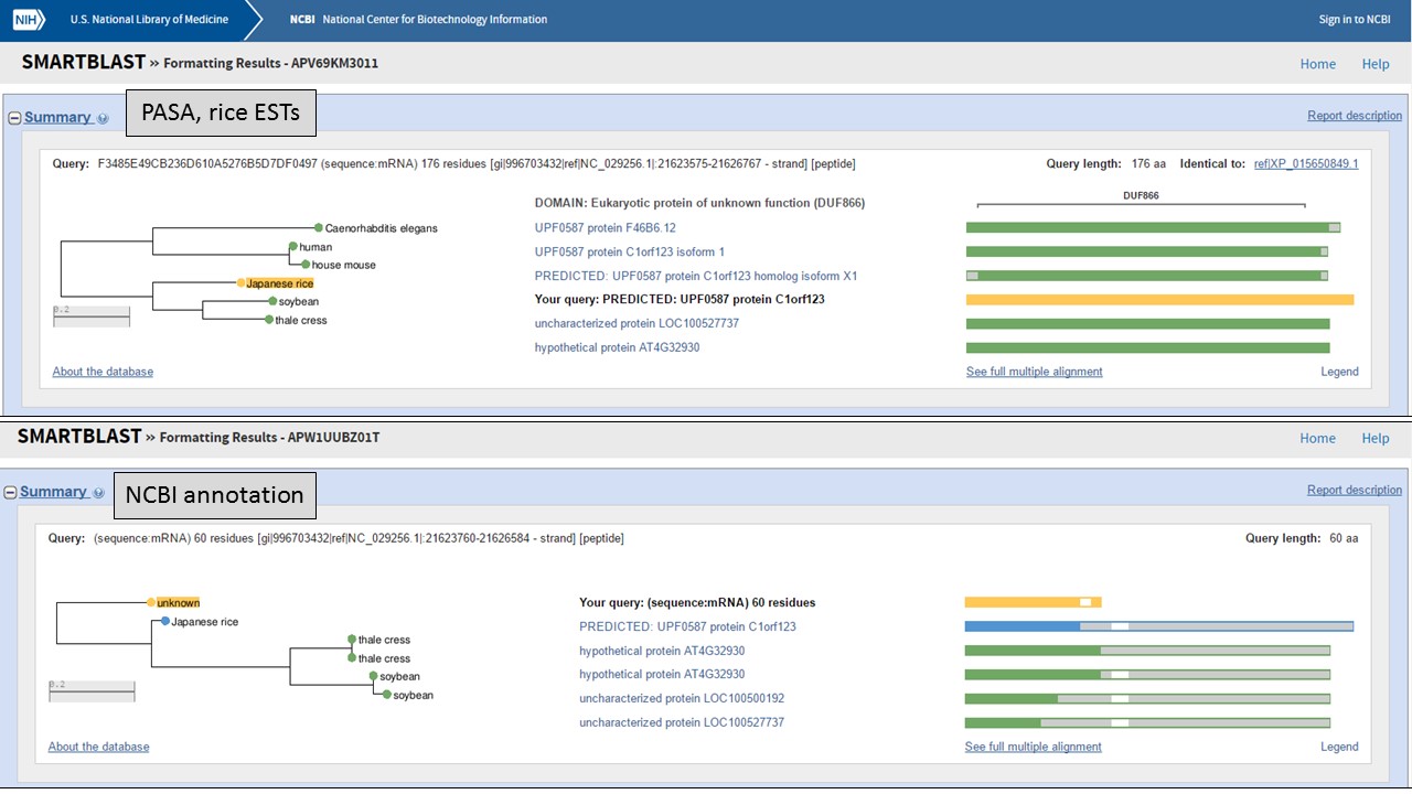
Figure 61. SmartBLAST results of proteins derived from gene models.
Since the "PASA, rice ESTs" gene model is supported by the evidence, the "NCBI annotation" gene model needs to be deleted from the "User-created annotations" track (see Fig. 54 above for instructions). We can now focus on the final edited gene model and can add information to the feature information. To do this, double-click the gene model to select it and then right-click and choose the "Information Editor" option (Fig. 62).
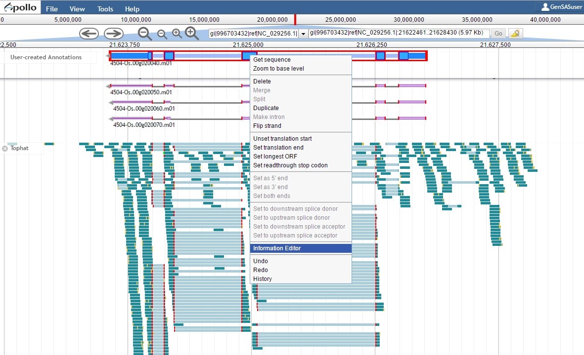
Figure 62. Opening the Information Editor window.
A pop-up window opens and has fields for the gene and mRNA annotations (Fig. 63). You can enter information in the boxes by clicking "Add" and then entering info into the field that appears.
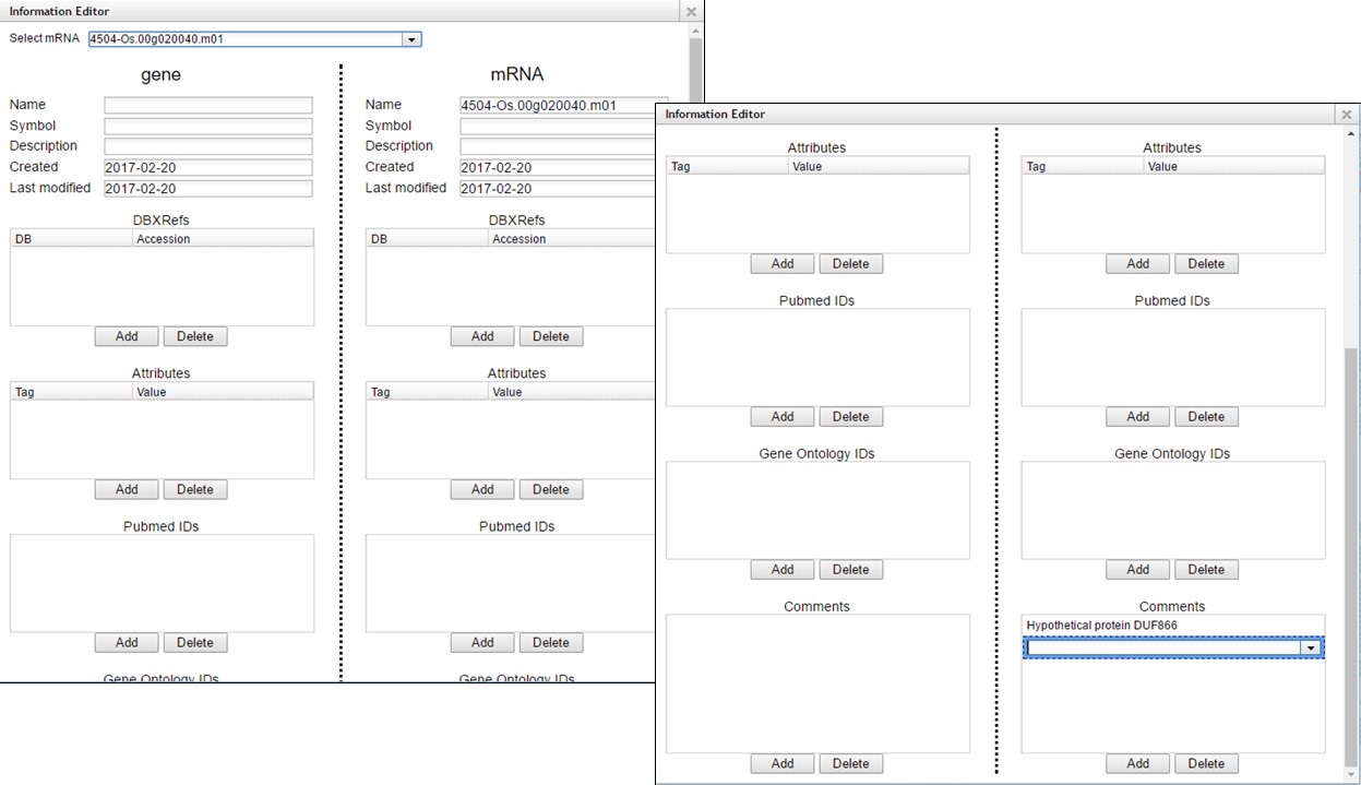
Figure 63. Information Editor window fields.
Once you have completed manual curation, you can prepare the final files by going to the "Publish" step.