GenSAS User's Guide
This User's Guide is designed to help you learn how to use GenSAS. The "Using GenSAS" section has very detailed instructions on how to use GenSAS. This section also was written for researchers who have never annotated a genome before and includes some suggestions on best practices. A video tutorial section with brief videos on how to use GenSAS will be coming soon. Please access these sections of the User's Guide by scrolling to the bottom of this page (under the flowcharts), or use the "GenSAS User's Guide" sidebar menu on the right to navigate through the sections of the User's Guide.
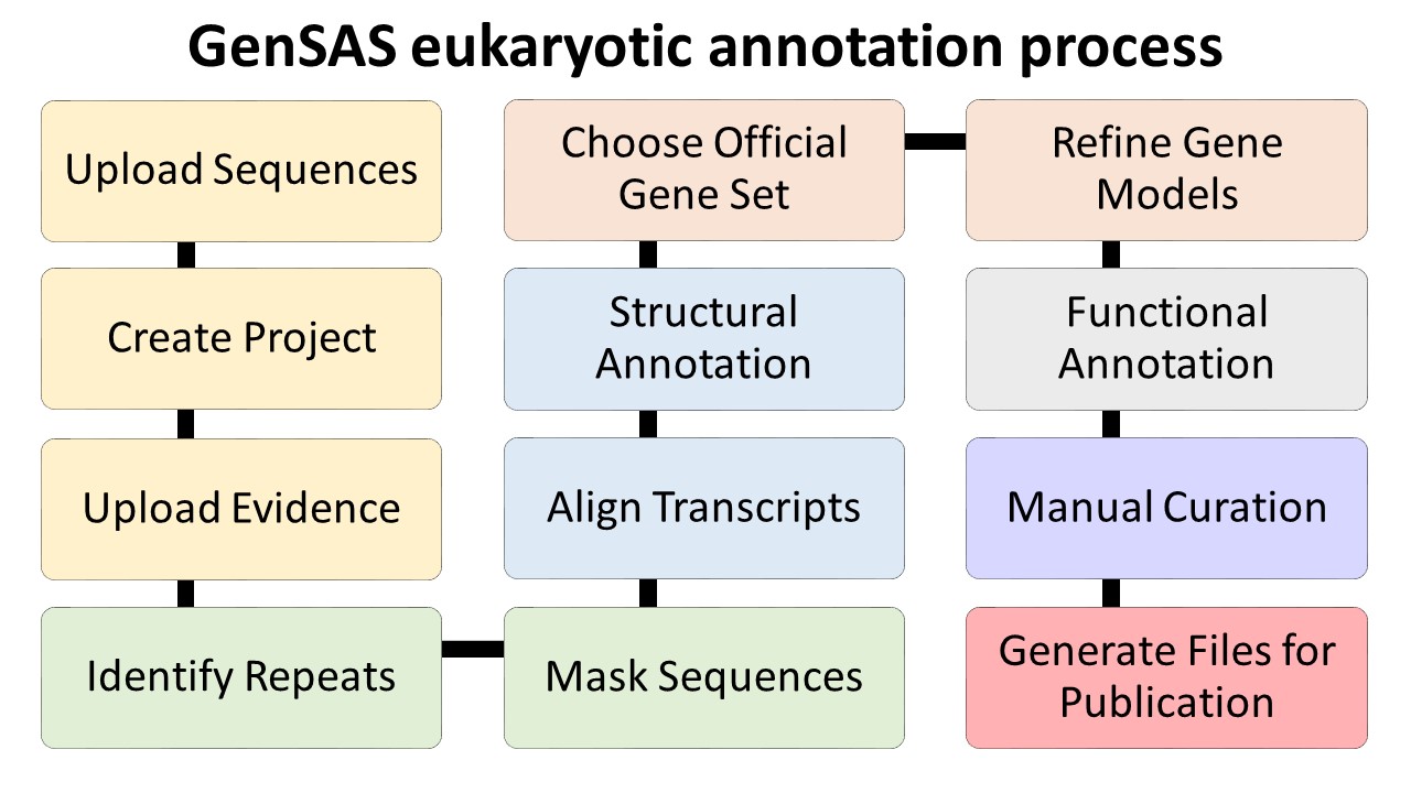
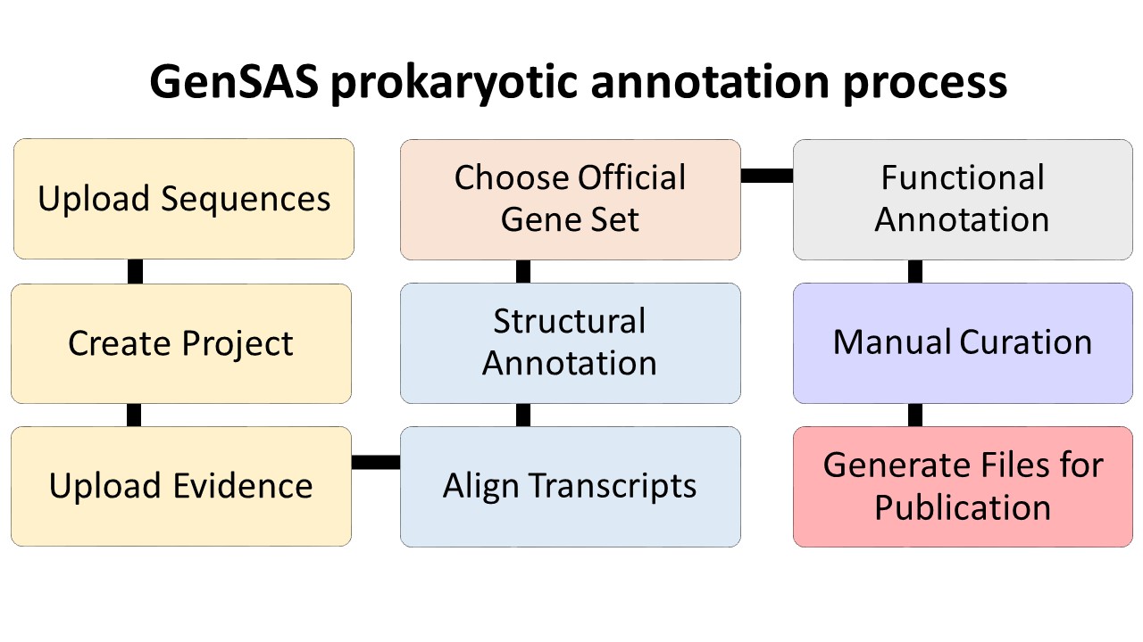
Please make sure that your genome is ready to annotate before loading it into GenSAS. Contigs that are smaller than the average gene size for an organism will not annotate properly with the provided tools. If your genome assembly is predominantly small contigs that are below the average gene size, then your genome probably will not annotate well with GenSAS. If you do not have the metrics of your assembly (i.e. N50, min/max contig size, number of contigs), please consider running the assembly file through a program (such as PRINSEQ) that will provide that data prior to loading it into GenSAS and please note the Project Limits in regards to the number and size of contigs in the assembly. Below are overview diagrams of the annotation process with eukaryotes and prokaryotes.
The steps on the flowcharts with the same color represent the major steps of annotation:
- Project creation/uploading sequences and evidence
- Repeat identification and masking (for eukaryotes)
- Structural annotation
- Selection of official gene set (and refinement for eukaryotes)
- Functional annotation
- Manual curation of the annotation
- Preparing files for publication
User Account and Project Limitations
GenSAS is currently available to use for free. The only requirement is to sign-up for a user account. The demand for GenSAS has been amazing and initially we had no limitations on project and uploaded assembly file sizes, but now that the number of GenSAS users have increased, we are implementing some limitations in order to make sure GenSAS has computational resources available to complete jobs and to allow the most users to use it effectively. Here are the limitations for GenSAS users:
- Only one account per user. Each user will only be allowed one account in order to keep resources available for all users. If we discover you have created a second account to bypass user limitations, you will be notified and one account and associated data will be deleted.
- GenSAS user accounts will remain active as long as users have an active GenSAS project. When users have let all their GenSAS projects expire, and have not logged into GenSAS for six months, their user account will be deleted to free up storage space on the server. Projects automatically expire after 60 days unless the user resets the expiration on the project.
- GenSAS users are limited to a total of 250 GB of storage space on GenSAS server. This size limit includes all user-uploaded assemblies and evidence files as well as all results files generated by GenSAS. This size limit is per user, not per project. When a user reaches the storage limit, they will be notified and will not be able to run any more GenSAS jobs until old projects are deleted.
- Assembly files must be high quality. GenSAS has been designed to annotate whole genome assemblies, not transcript assemblies. Assembly files that are loaded under the "Sequences" step are analyzed using PRINSEQ. Assembly files must contain less than 25,000 total sequences and more than 50% of the sequences must be over 2500 bases in length. Uploaded files that do not meet these requirements will not be available for use in GenSAS projects.
- Users can only have seven running jobs at a time. GenSAS users are limited to seven actively running jobs at a time, across all projects. However, users can set-up more than seven jobs and have the jobs waiting in the job queue. As jobs complete, the waiting jobs will be submitted.
- GenSAS projects are not backed up and GenSAS is not a data storage solution for your files. While data loss is rare, it can happen. We highly recommend downloading your final annotation files from GenSAS when your project is complete as well as keeping copies of the assembly and evidence files you uploaded. Users who continually renew projects with no evidence of actively running jobs, will have their projects removed to make space for new users and jobs. You will be notified about the eventual file removal and be given a short time frame to download your files.
Using GenSAS
GenSAS utilizes user-friendly interfaces and embedded instructions to guide the user through the annotation process. This User Guide will describe the use of each section in more detail. Please also see the video tutorial section (coming soon).
GenSAS performs structural and functional annotations of whole genome assemblies or single DNA sequences. If you have never performed DNA annotation, we recommend reading "A beginner's guide to eukaryotic genome annotation" as a starting point to familiarize yourself with the overall process. GenSAS requires user-interaction for the annotation process. We have included very basic descriptions of how to use the tools which are integrated into GenSAS, but if you would like to know more specifics about each tool, please see the "Available Tools" table on the homepage and visit the websites for the tools to see detailed documentation.
GenSAS Homepage
The GenSAS hompage is the access portal for using GenSAS and also has other useful information. On the right side, is a place to login to GenSAS (Fig. 1A). If you do not have an account, please use the link to request an account. Please note that account requests are reviewed prior to approval and are not automatic. Account requests are usually approved within 24 hours. If you have an account, and have forgotten your password, there is a link to request a new password. Once logged into GenSAS, your account information can be edited by clicking on "My account" in the upper right corner.
.jpg)
Figure 1. The GenSAS homepage.
In the header of the homepage, are a series of tabs (Fig. 1B). Once logged in, click on the "Use GenSAS" tab to go to the GenSAS interface. To view the available tools, click on the "Available Tools" tab. On the Available Tools table, there are hyperlinks to the websites for each tool available in GenSAS (Fig. 2A). GenSAS provides the RefSeq, SwissProt, and TrEMBL databases as well as the RepBase repeat libraries. Information on the globally provided data, and the release dates, can be found on the "Available Libraries" tab (Fig. 2B). To contact GenSAS support, read the User's Guide, and view the video tutorials click on the "Help" tab. Finally, to find a citation for GenSAS, please click on "Cite GenSAS."
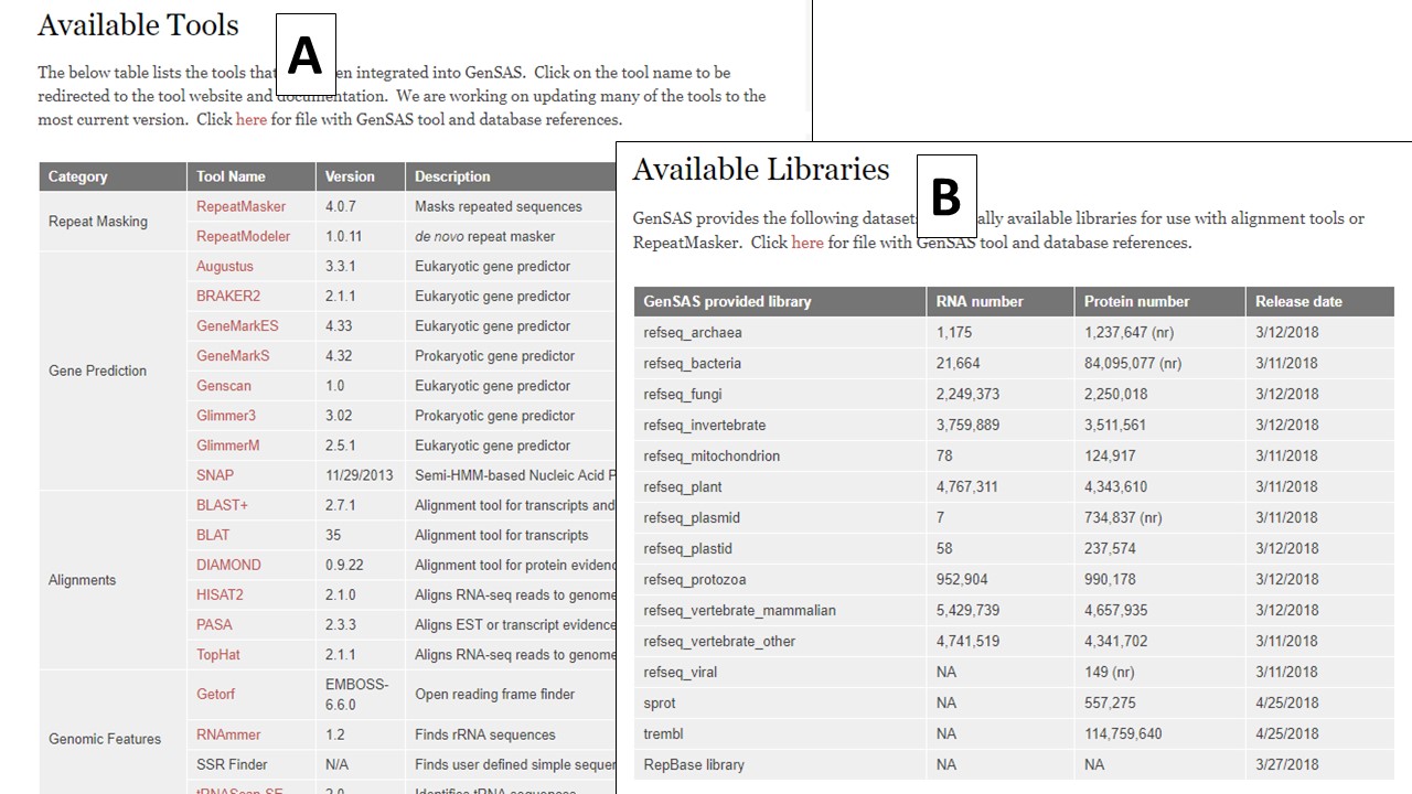
Figure 2. The tools and databases available in GenSAS.
GenSAS Interface
The GenSAS interface has three main sections. The header region (Fig. 3A) has a flowchart of the annotation process. Annotation steps that are available for use have blue arrows, the step that you are currently viewing has a green arrow, and steps that are not yet available have grey arrows. Clicking on the blue or green colored arrows will open the tab for that step of the annotation process. The header also displays the name of the project that is open in the upper left corner and in the upper right corner is the user name and links to account info, the GenSAS homepage, and to logout.
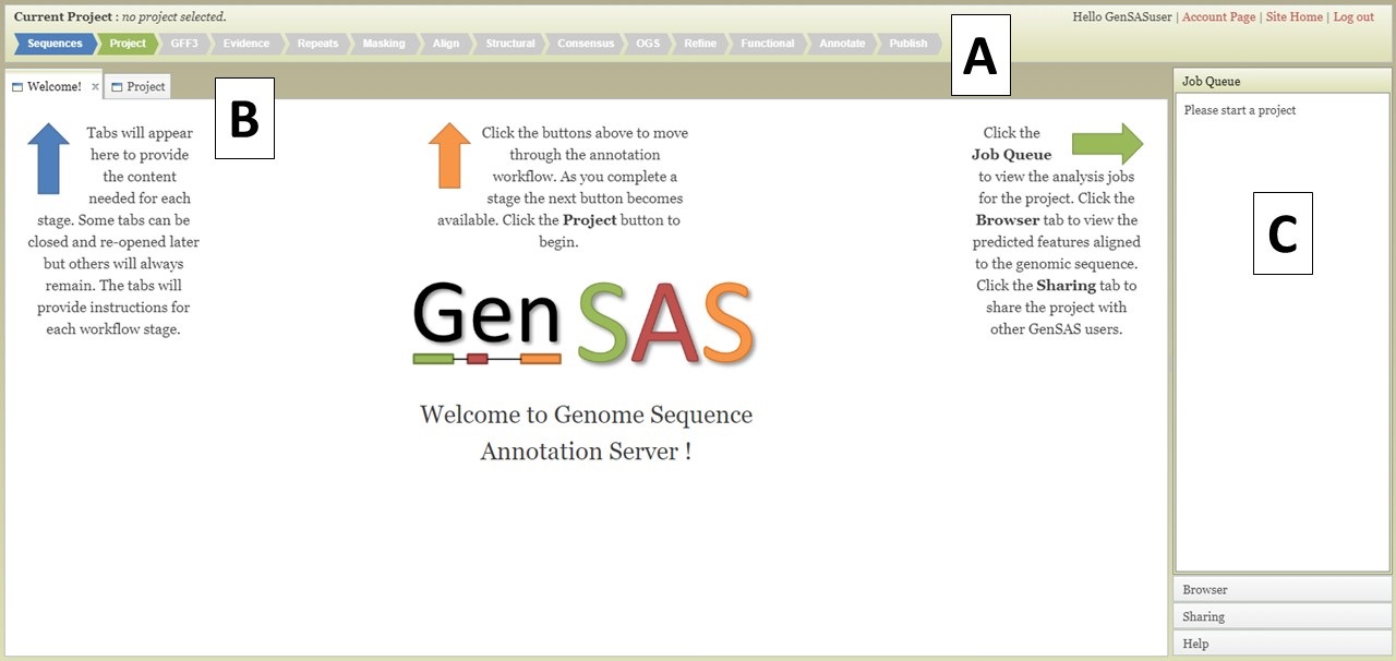
Figure 3. The GenSAS interface.
The center part of the GenSAS interface is the tab area (Fig. 3B). This is the main area where user interaction happens and each step of the annotation process has a tab where jobs can be created. This is the also the area where tabs will open to show job results, to use Apollo, and to view results in JBrowse. More details on the content of the tabs will be covered in the other sections of this guide.
GenSAS has an accordian menu on the right side that has four sections (Fig. 3C). When a project is loaded, the "Job Queue" section will show a list of all jobs that are associated with the project and their status. Once jobs are submitted in GenSAS, you can log out. Jobs will continue to run, and progress will automatically be saved. If you would like to see where your jobs are at in the queue to run on the server, click "View Full Report" at the top of the Job Queue to see more details about each job. Please note that each user may only run seven jobs at one time, across all projects. If more than seven jobs are submitted, the extra jobs will be in "waiting" status until previous jobs finish. If you want to refresh the current run status of jobs, click on "Update status" at top of job queue. The "Browser" section is used to open the Apollo tab (see "Apollo and JBrowse" section for more info). The option to open the browser is only available after the first job associated with the project has completed. The "Sharing" section is for sharing GenSAS projects with another user. Projects can only be shared after there is a completed job for the project (see "Sharing Projects" section for more info). And the last section is the "Help" section. In this section there are links to the User's Guide, troubleshooting, and a link to contact us.
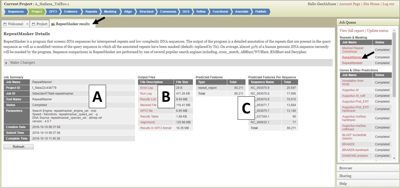
Figure 4. The GenSAS Job Queue.
Clicking on the job name in the Job Queue opens a tab with details about that job (Fig. 4). There is a summary of the job settings in a table on the left (Fig. 4A), and log files and raw result files are in a table in the center (Fig. 4B). The log and raw result files can be downloaded by clicking on the names in the table. On the right, are summary tables listing how many features were annotated by the tool (Fig. 4C). Please do not rely solely on seeing numbers in these tables for the structural annotation tools. Please look at the data in JBrowse to determine if the results make sense before proceeding to the next step. The total number of features from functional annotation tools will not be reported in the Predicted Features tables. For functional annotation results, there will be an additional table with the names of each gene model that returned functional tool results.
Sequences Tab
The first step to use GenSAS is to add the sequences you would like to annotate. Please note that GenSAS is designed to annotate whole-genome assemblies, not transcript assemblies. Sequence files uploaded to GenSAS must contain less than 25,000 individual sequences and over 50% of those sequences must be over 2,500 bases in length. When you open the GenSAS interface, you will see the welcome tab. The "Sequences" and "Project" tabs on the flowchart in the header will also be available to click. To add sequences, click on "Sequences" in the flowchart in the header. Sequences that are added to GenSAS are associated with your user account and once added, and processed, are available to use in a GenSAS project. All GenSAS tabs have an instructions section (Fig. 5A) that can be viewed or hidden by clicking on "Instructions." The embedded GenSAS instructions contain a basic overview on how to use that part of GenSAS and more detailed instructions are found in this User's Guide.
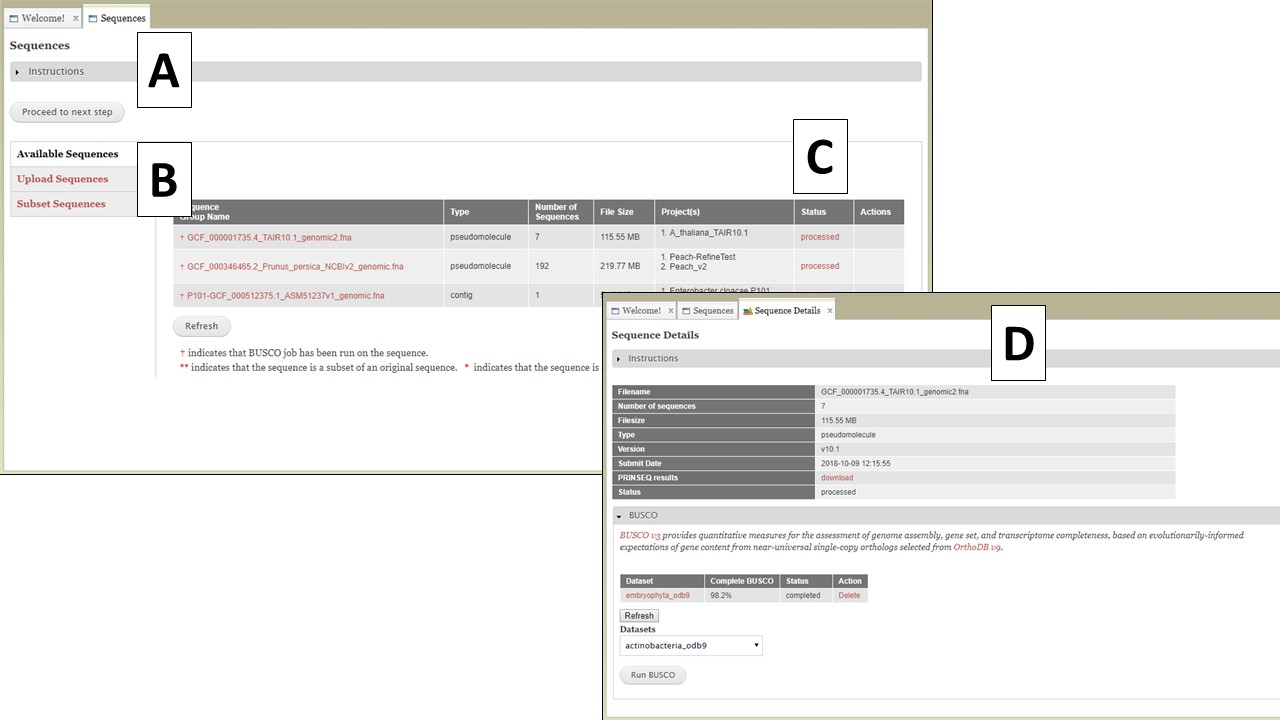
Figure 5. The Sequences tab in GenSAS.
The Sequences tab has three options listed on the right (Fig. 5B); Available Sequences, Upload Sequences, and Subset Sequences. The tab automatically defaults to "Available Sequences" and displays a table of all the sequence groups that are associated with your user account (Fig. 5C). After uploading the file, GenSAS needs time to process the file before it appears on the sequence table, and is available for use in a project. GenSAS checks the file and determines the number of sequences and the size of the sequences. Files that have "violated" the minimum requirements are marked as such under the "Status" column on the table. Clicking on the sequence file name will bring up a summary of the file pre-screening (Fig. 5D). If the sequence file did not pass the screening process, the option to use only the sequences above 2,500 bp in length is available. If the sequence has passed the pre-screening, the option to run BUSCO is available (Fig. 5D). All sequences that are loaded from a multiple-sequence FASTA file are considered to be a single "sequence group." When a sequence group is used in a GenSAS project, all sequences are processed by the annotation tools. The option to remove a sequence group from your user account is only an option if the sequence group is not part of an active GenSAS project. If the sequence can be deleted, the "Delete" button appears in the "Actions" column of the table.
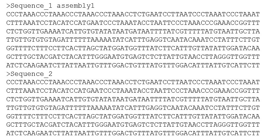
Figure 6. An example of the FASTA file format.
All sequences that are added to GenSAS must be in the FASTA format (Fig. 6). The FASTA format is a very common file format for DNA and protein sequences. The file extension can be one of the following: .fa, .fas, or .fasta. Please do not use spaces in your file names. Replace spaces with underscores or dashes. Within a FASTA file, the sequence name is on a line and starts with a ">". The sequence is then on a new line, immediately after the sequence name and does not have any special characters. A file with multiple sequences should have the next sequence right after the end of the first sequence without an empty line in between them (4 lines total in this example). Please note that any information following the first space in the sequence name will be removed. In Fig. 6, the first sequence is called "Sequence_1 assembly1". In GenSAS, the name will be truncated to "Sequence_1". If the sequence names in this example were missing the underscore in "Sequence_1" and "Sequence_2" and used a space instead, then the sequence names would both be "Sequence" in GenSAS during annotation and at the end when GenSAS produces the final annotation results. Please make sure that your sequences have unique names so the data generated with GenSAS is useful at the end.
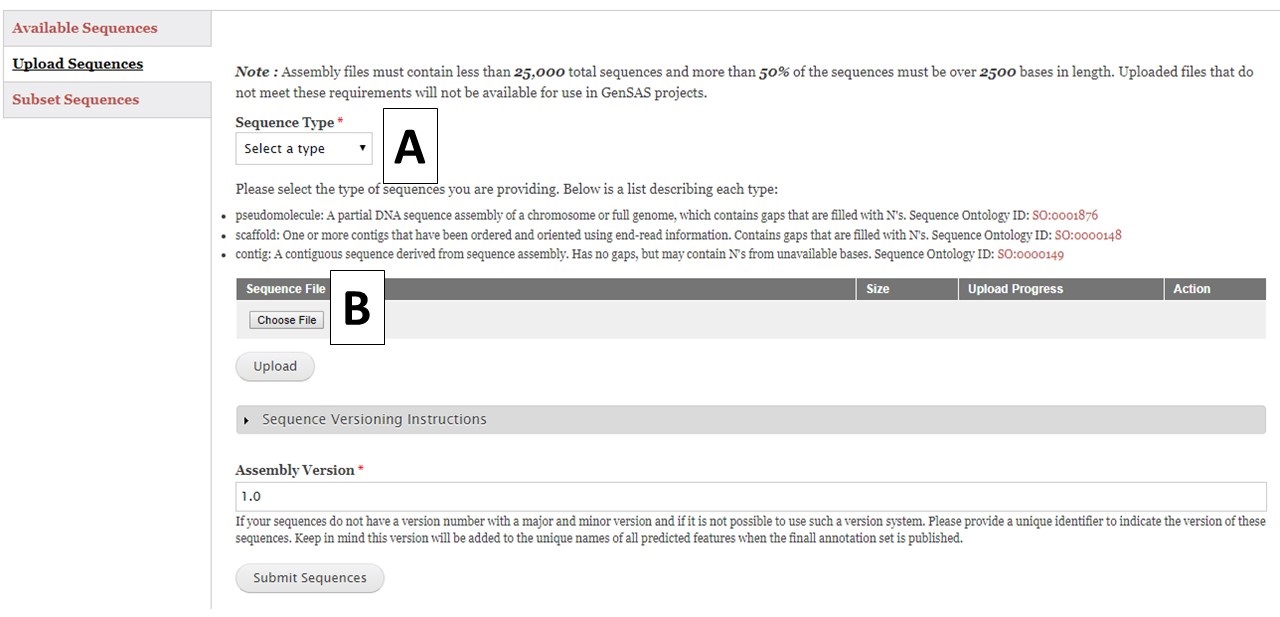
Figure 7. Upload Sequences section of Sequences tab.
To upload sequences, select the sequence type (Fig. 7A) and then choose a single file (Fig. 7B) and click "Upload". While the file is uploading, complete the rest of the webform with the information about the assembly version number. GenSAS will add the assembly and annotation version numbers to the output files during the "Publish" step. Then check on the progress of the file upload. Once the file has successfully uploaded, click the "Submit Sequences" button at the bottom of the page to add your sequences to GenSAS. If you do not click "Submit Sequences," the files will not be added. Please note that after submitting sequences to GenSAS, the file is processed by GenSAS and it make take awhile before the file appears in the "Available Sequences" section (especially true for large sequence files). The Sequence Group will not be available for use in a project until it appears on the table.
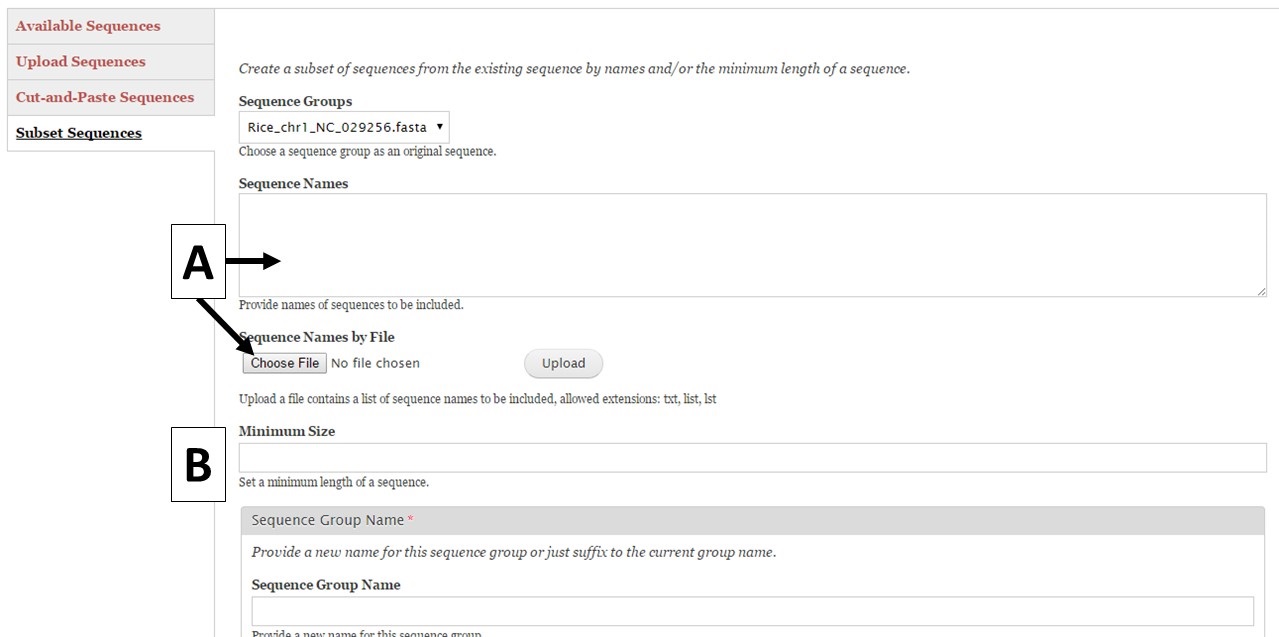
Figure 8. Subset Sequences section of Sequences tab.
GenSAS also has the ability to create sequence subsets from any Sequence Group with multiple sequences. If you are doing a whole genome annotation, or other project with numerous contigs or scaffolds, we highly recommend trying out GenSAS on a smaller subset of sequences so you can optimize the tools settings and can determine which tools work best for your DNA sequences prior to annotating the whole genome. Sequence subsets can be created using the "Subset Sequences" option (Fig. 8). To create a subset, choose the Sequence Group from your previously uploaded sequences using the drop-down menu. You can then filter out sequences by sequence name (Fig. 8A) or minimum size (Fig. 8B). The sequence names can either be entered in the text box, or you can upload a text file of sequence names (one sequence name per line). After setting the filtering options, provide a name for the sequence subset and click "Subset Sequences." Sequence groups created using "Subset Sequences" are shown in the Subset sequences table in the "Available Sequences" section (Fig. 9A). Once the subset appears on this table, the sequence group can be used in a GenSAS project.
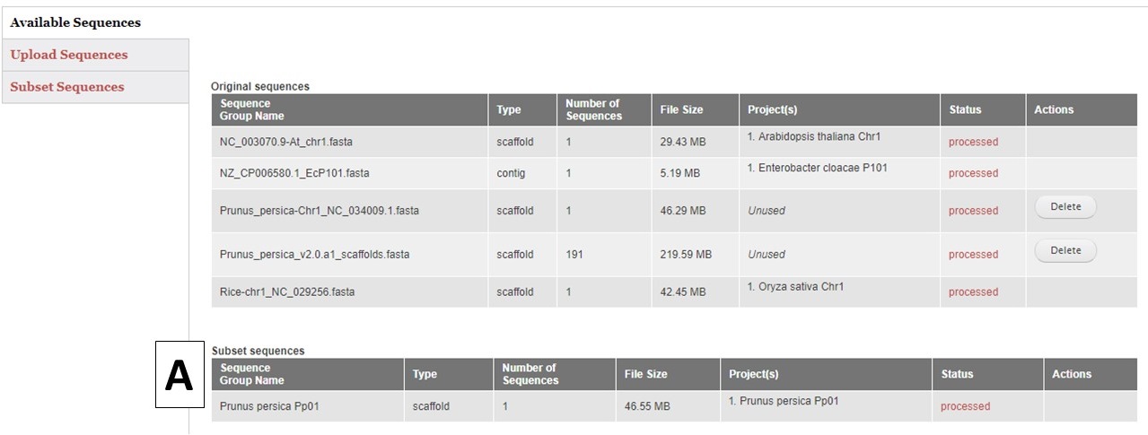
Figure 9. Subset Sequences that are available for use in GenSAS.
If you also have chloroplast, mitochondria, plastid, or plasmid DNA as scaffolds in your eurkaryotic genome project, we recommend separating those sequences out into indiividual projects so they will be annotated with tools more appropriate for those DNA types.
Project Tab
The Project tab is used to either open existing projects or to create a new project in GenSAS. To load an existing project you created, or a GenSAS project that has been shared with you, select the project from the pull-down menu on the "Load an Existing Project" section (Fig. 10A). To start a new project, select the "Begin a New Project" option (Fig. 10B). For new projects, there is a webform with required and optional information fields. You will be required to enter a project name, the type of organism, genus, and species along with selecting the Sequence Group for the project. The other fields are optional, and are mainly there for the user to help manage their projects. At the bottom of the webform, is the option to receive emails from GenSAS when jobs start and finish. You can choose to turn these emails on or off. Make sure to click "Create Project" when you are done.
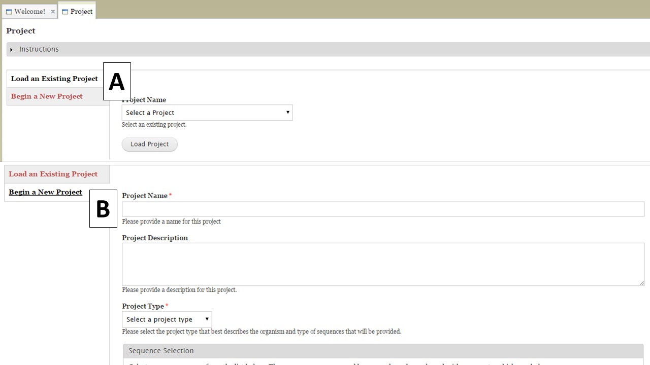
Figure 10. Project tab in GenSAS.
Once a project is created, or a previous project is opened, the Project Summary is displayed on the Project tab (Fig. 11). Please note that all GenSAS projects expire after 60 days unless the user renews the project. You will receive several email reminders as the project expiration date gets closer. To ensure that your GenSAS project does not get deleted after 60 days, open the project and click the "Reset Expiration" button (Fig. 11A) located at the top of the Project Summary info before the project expires. You can also delete a project by clicking the "Delete this Project" button on the Project Summary page. If you want to switch projects in GenSAS, simply click the "Close this Project" button on the Project Summary and the options to open another project or start a new one will appear. If you would like to edit the project and organism details, choose the "Edit Project" option (Fig. 11B) from this summary page.
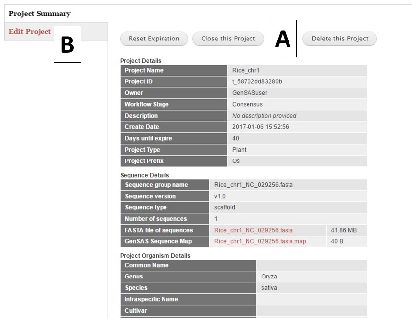
Figure 11. Project Summary table on Project tab.
GFF3 Tab
If you have a previous annotation, or results from other annotation tools, in the GFF3 format, the results can be uploaded to GenSAS and used during the annotation process. The GFF3 format is a standard 9-column file that has specific information in each column. Basically a GFF3 file lists the locations of features (genes, alignments, repeats) on a specific DNA sequence. GFF3 files must have been created from the sequence you uploaded into GenSAS. For more details about the GFF3 format, please see the GMOD wiki. For GenSAS, it is important to make sure that the sequence names in column 1 of the imported GFF3 file, exactly match the sequence name being used in GenSAS (Fig. 12). Please see the information about sequence names in GenSAS on the Sequences Tab page in this guide. If the sequence names in column 1 of the GFF3 file do not match the sequence names in GenSAS, then the data will not be imported into GenSAS.
.jpg)
Figure 12. Example of GFF3 file format.
There are five different GFF3 file import options; Repeats, Transcript Alignments, Protein Alignments, Gene Predictions, and Other Features (Fig. 13). Each importer will recognize and import certain feature types in the GFF3 file (Table 1). Feature types are listed in column 3 of the GFF3 file. All imported GFF3 data can be viewed in JBrowse, but some of the data can also be used during the annotation process. For example, the repeat data will be available under the Masking step and the transcript data will be available for use to make a gene model consensus. The "GFF3 Files" option (Fig. 13A) will display a list of all GFF3 files that have been uploaded by the user and whether they are use in the current project or other projects. Files that are not in use, can be deleted by the user.
| GFF3 Importer | Recognized feature types |
|---|---|
| Repeats | repeat, repeat_region |
| Transcript Alignments | match, match_part |
| Protein Alignments | match, match_part |
| Gene Predictions | gene (required), transcript, mRNA, CDS, exon, five_prime_UTR, three_prime_UTR |
| Other Features | any term in column 3 |
Table 1. GFF3 feature types recognized by the GFF3 importers in GenSAS.
To import a GFF3 file, click on the appropriate importer for the data type you are uploading. Use the "Choose File" option to select a new GFF3 file and then click "Upload"(Fig. 13B). If the GFF3 file has been previously loaded into GenSAS, use the pull-down menu under "GFF3 File" (Fig. 13C) to select the file. Type in a Job Name and click "Import File" and a job will appear in the Job Queue. If you have different GFF3 files to load under the same importer type, you can set-up multiple jobs. Each job uploads a single file, and each job must have an unique name. Please make sure your job names are meaningful so you know what data was imported by that job when viewing the data later in GenSAS.
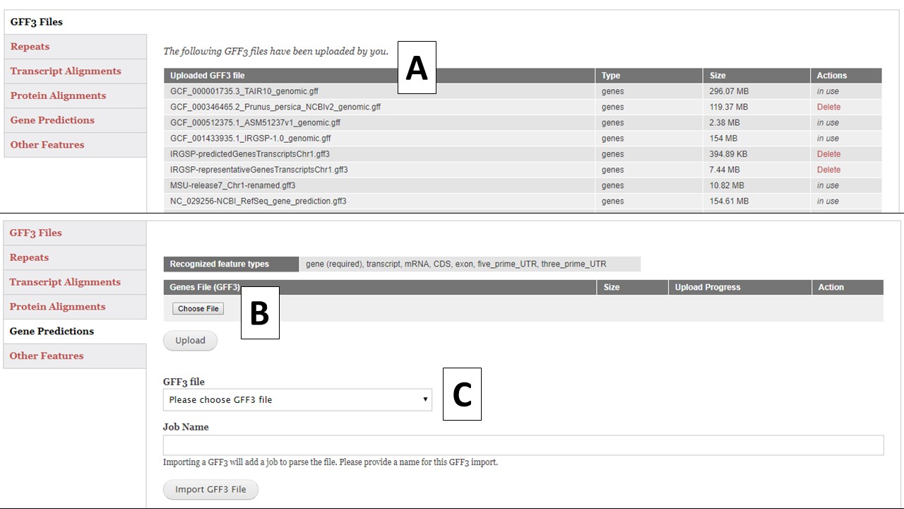
Figure 13. GFF3 tab in GenSAS.
Once you have submitted the import jobs, GenSAS will process the files and once the jobs are complete, you will be able to open JBrowse and view the data. Open JBrowse by clicking on the "Browser" link in the right hand menu and then click "Open Apollo". When you are done uploading GFF3 files, click "Proceed to next step", which is located near the top of the tab, to move on to the next step of the annotation process.
If your GFF file is a eukaryote based genome project which also includes chloroplast, mitochondria, plastid, or plasmid DNA as scaffolds please be aware that the gene models for those sequences will not import into JBrowse. For eukaryote projects, GenSAS displays mRNA features in JBrowse/Apollo. These sequences are prokaryotic in origin and usually do not have mRNA features in the annotations.
Evidence Tab
Under the Evidence tab, you can upload evidence files that will be accessible to several tools during the annotation process. Please use data from your species for the best results, but if data from your species is not available, data from a very closely-related species can be used. There are five different evidence types that can be loaded into GenSAS (Fig. 14A). The interface to upload each data type is accessed by clicking on the name (see more details below). The Evidence tab defaults to the "Evidence Files" section that has a table of all evidence files that are associated with your user account (Fig. 14B). If you have uploaded files under another project, they will be available to use in all projects associated with your GenSAS account. As files are uploaded using this tab, you will have to click "Refresh table" (Fig. 14C) to see the files. Files only appear on this table when the upload to GenSAS is complete. Please do not close your browser or log out of GenSAS until the file upload(s) is complete. Large files (i.e. RNA-seq reads) will take a long time to upload.
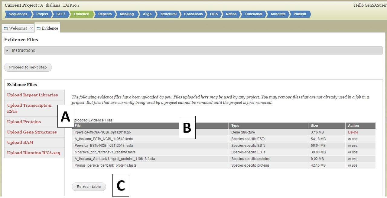
Figure 14. Evidence tab in GenSAS
For the different evidence categories, different file types are accepted. For Repeat Libraries, Transcripts & ESTs, and Proteins, FASTA file formats are accepted. Please see more about the FASTA format under the Sequences section of the User Guide. For the Gene Structures category, a Genbank (.gb) file format is accepted and can be used to train Augustus. For the Genbank gene file, there must be at least 100 sequences in the file for Augustus to use the file during training. BAM files of aligned RNA-seq reads can also be uploaded and used to train Augustus and BRAKER. To add files, click on the appropriate category (Fig. 15A), click on the "Choose File" button to select the file and then click "Upload Files" (Fig. 15B) to start the upload process. You will then see a progress bar appear on the table (Fig. 15C). Do not close your browser or logout of GenSAS until the process has completed. If you close your browser, then the file upload process stops. Once the file has uploaded, you can view the file on the table in the "Evidence Files" section by clicking on "Refresh table" (Fig. 14C).
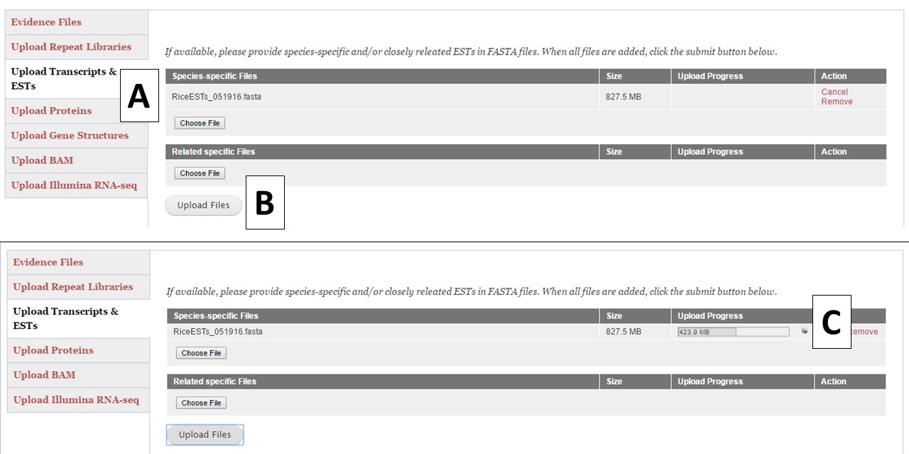
Figure 15. Example file loading process.
Under the "Upload Illumina RNA-seq" section you can upload pre-processed RNA-seq reads from the Illumina platform (Fig. 16). GenSAS currently only supports reads from Illumina. We also ask that the reads have been at least filtered to remove any low-quality reads. You are allowed to load up to 100 GB of RNA-seq data either as a single set of paired reads (Fig. 16A) or one non-paired reads file (Fig. 16B). Please be aware that the upload process may take a significant amount of time due to the file sizes. You may want to consider only loading a portion of your RNA-seq reads into GenSAS. Please note that GenSAS is not a tool for analyzing RNA-seq data. If you are having problems with getting your RNA-seq data uploaded (files > 2 Gb in size) to GenSAS, please contact us. The RNA-seq reads can be aligned to your genome with TopHat and the resulting alignment can be used to train gene model prediction programs. You can also upload assembled RNA-seq data as a FASTA file under the "Upload Transcripts & ESTs" section to use with the other alignment tools in GenSAS.
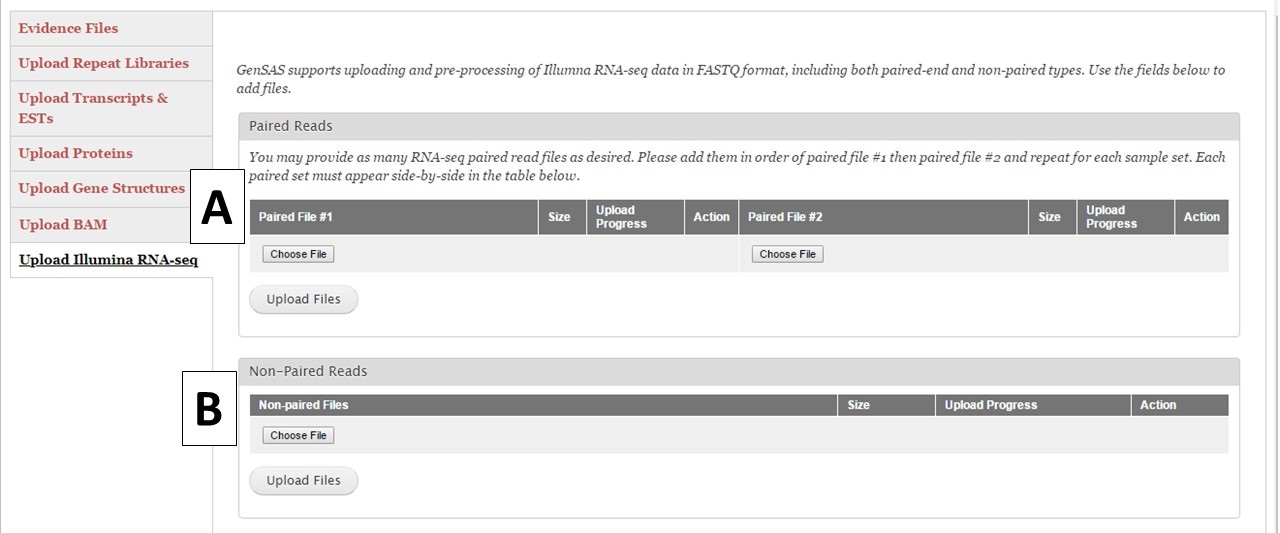
Figure 16. RNA-Seq read upload interface.
When you are done uploading evidence files, click "Proceed to next step", which is located near the top of the tab, to move on to the next step of the annotation process.
Repeats Tab
Under the Repeats tab, you will run tools to mask repeats in the genome sequence. The Repeats tab is only available to eukaryotic organisms. If you are working on a project of the project types: bacteria, archaea, mitochondrion, plasmid, plastid, or virus; the Repeats and Masking steps are not available for use since the DNA sequences are of the prokaryote type and do not require masking. Repeats are masked during eukaryotic DNA annotation in order to mask the repetitive sequences and allow downstream annotation tools to focus on the more likely gene encoding regions. You can choose to skip repeat masking in GenSAS and in that case, the original un-masked sequence will be used. There are two repeat finders in GenSAS: RepeatMasker and RepeatModeler (Fig. 17A). Repeatmasker relies on evidence or pre-determined repeat libraries for organisms, whereas RepeatModeler is a de novo repeat finder. Please see the "Available Tools" table for details about these tools.
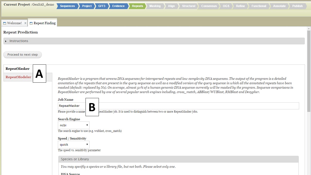
Figure 17. Repeats tab in GenSAS.
For RepeatMasker, there are settings that can be adjusted by the user. You can run more than one RepeatMasker job, with different settings, as long as you provide unique job names (Fig. 17B). GenSAS provides the organism specific repeats from Repbase and the files can be selected under the "Species or Library" option of the RepeatMasker section (Fig. 18A). If you uploaded a FASTA file under the Evidence tab, you will see your file under the "Repeat Library" option (Fig. 18B). The rest of the settings are automatically set to the default parameters for RepeatMasker, but you may change the settings. Please read the documentation for RepeatMasker and understand what each setting does before making changes to these. Once the settings are set, click on the "Add RepeatMasker Job" button. You should see the job name appear in the job queue (Fig. 19B).
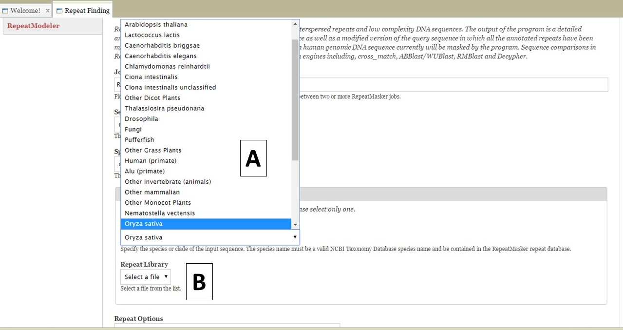
Figure 18. RepeatMasker settings.
For RepeatModeler, there are no settings to set since it is a de novo repeat finder. To add a RepeatModeler job, simply click the "Add RepeatModeler Job" button (Fig. 19A). Once the job is added, the job name will appear in the Job Queue (Fig. 19B) on the right side of the GenSAS interface. You will have to wait for the repeat masking jobs to finish before you can use the next step of GenSAS, but to move to the Masking step of GenSAS, click on the "Proceed to next step button" under the instructions section.
.jpg)
Figure 19. RepeatModeler and Job Queue.
Apollo and JBrowse
Once you have completed jobs in the job queue, you can view the results by clicking on the job name in the Job Queue (details in GenSAS Interface section), or you can view the job results in JBrowse. JBrowse and Apollo (a JBrowse plugin) are integrated into GenSAS and are accessed by clicking on "Browser" in the right hand accoridan menu (Fig. 20A). Once the Browser section of the menu is open, you will see the "Open Apollo" button (Fig. 20B). When that button is clicked, an Apollo tab opens. You can find more detailed information about Apollo and JBrowse through the links on the "Available Tools" table. Please remember that larger genomes take longer to load into JBrowse, please be patient.
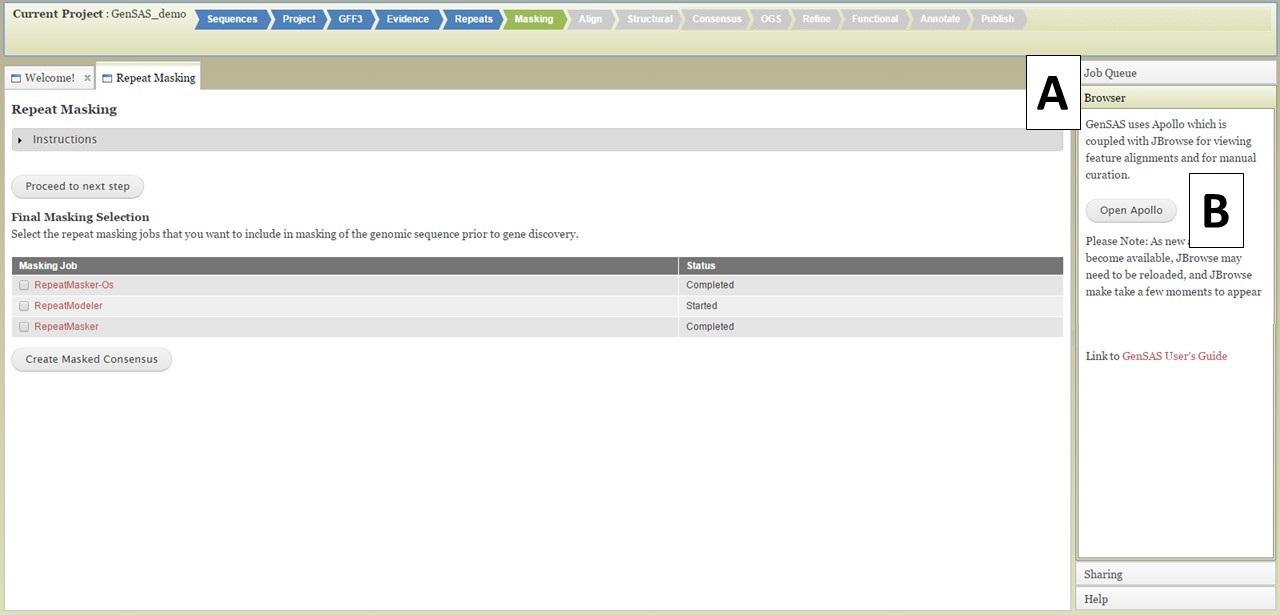
Figure 20. Opening Apollo/JBrowse with Browser section of GenSAS accordian menu.
There are two sections of the Apollo/JBrowse interface with in the Apollo tab. On the left is the JBrowse section and on the right is the Apollo section (Fig. 21). The divider between the two sections can be moved left or right to adjust what is viewable on each side (Fig. 21A). When you open Apollo/JBrowse for the first time, no tracks will be visible. Your browser cache will remember the Apollo/JBrowse settings when you open the Apollo tab again later. To make the tracks visible, click on the "Tracks" tab within the Apollo interface (Fig. 21B), and then expand the track categories and click on "show" by the track names (Fig. 21C). The JBrowse track selection sidebar can also be enabled/disabled by clicking on "JBrowse TrackSelector" in the upper right corner of the Tracks tab in the Apollo section (Fig. 21D).
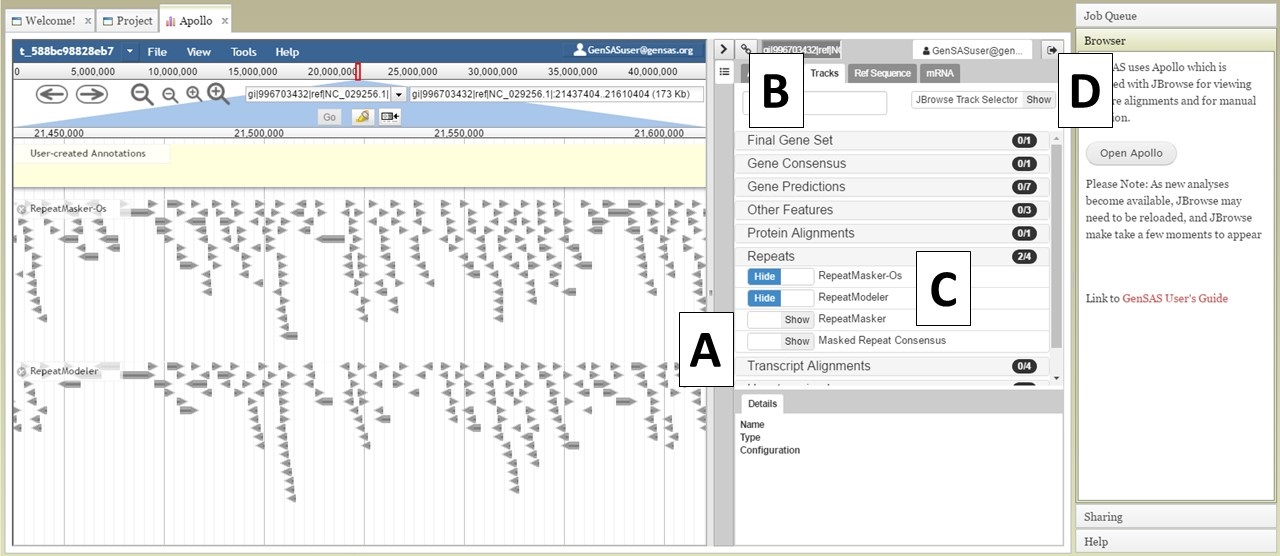
Figure 21. Apollo Tab in GenSAS.
At the top of the JBrowse window, there is a blue toolbar with a graphical represntation of the length of sequence and some contols below that (Fig. 22A). For a project with multiple sequences, only one sequence is displayed at a time. To change to another sequence in the JBrowse window, you can select from the pull down menu (first 30 sequences only) or you can type in the sequence name in the text box (Fig. 22B) and click "Go." You can also change sequences by using the "Ref Sequence" tab in the Apollo window (Fig. 22C).
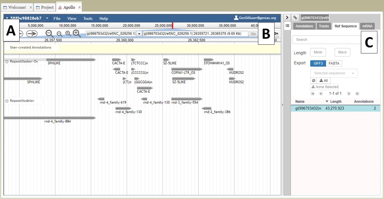
Figure 22. Navigating to different sequences in JBrowse/Apollo.
If you would like to hide the track names in JBrowse, click on the icon that has a box and arrow (Fig. 23A). If you right-click on the track name, track specific options will be available in a menu (Fig. 23B). If you would like to export a region of the track data, that can be done my selecting the "Save track data" option. You can also view details/edit information for a feature on the tracks by selecting and right-clicking on the feature (Fig. 23C).
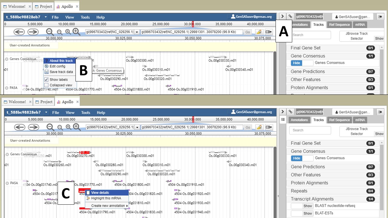
Figure 23. JBrowse functions.
You can also zoom and pan the view in JBrowse. You can use the arrows and magnifying glass icons in the JBrowse header to shift the view left and right and zoom in and out, respectively (Fig. 24A). If you zoom in all the way, you can even see the genome sequence (Fig. 24B). You can also shift the view in the window by clicking and dragging.
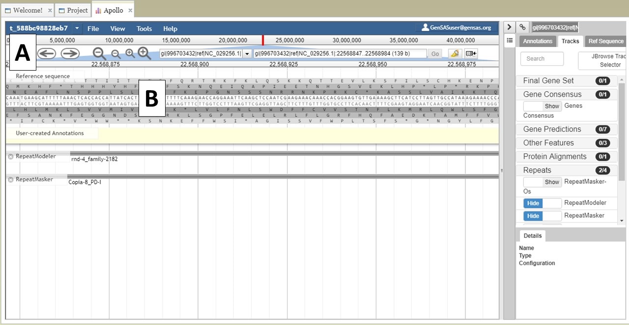
Figure 24. More JBrowse functions.
We will talk more about JBrowse and Apollo functionality in the "Annotate Tab" section of the User Guide. Please use JBrowse to view the results from the annotation tools and make sure the results make sense for your genome before using the data in downstream tools in the pipeline. If a tool does not return good results, it may affect the results of the downstream tool.
Masking Tab
Once the repeat finding jobs are done, it is very important to look at the repeat tool data (see "Apollo and JBrowse" section) before using the Masking tab. On the Masking Tab you will see a table with all repeat data in GenSAS for the genome (Fig. 25). You will need to decide if you want to use the results from one tool, combine the results from multiple tools, or to use unmasked sequences for the annotation process. The Masking tab is only available to eukaryotic organisms. If you are working on a project of the project types: bacteria, archaea, mitochondrion, plasmid, plastid, or virus; the Masking step is not available since the DNA sequences are of the prokaryote type and do not require masking.
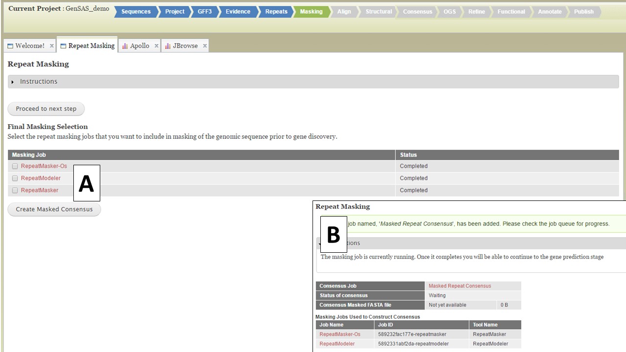
Figure 25. Masking Tab in GenSAS.
If you want to use a single set of data, select that dataset and click "Create Masked Consensus" (Fig. 25A) If you want to combine more than one dataset into a single masked consensus sequence, select the datasets you want to use and click "Create Masked Consensus." For both cases, a Masked Consensus job will appear in the Job Queue and a summary screen appears (Fig. 25B). Once the consensus job completes, the "Align" step will become vailable to use and all the downstream tools will use the masked sequence as input.. If you want to use unmasked sequences, just click on the "Proceed to next step" button and the original sequences will be used for the next steps.
Align Tab
Under the Align tab, you will be able to align RNA and protein evidence against the genome you are annotating. For eukaryotes, nucleotide BLAST, BLAT, HISAT2, PASA, and TopHat are available to use for transcript (nucleotide) alignments and protein BLAST and DIAMOND for protein alignments (Fig. 26). For prokaryote projects, nucleotide and protein BLAST are available along with BLAT. The page defaults to displaying the "Transcript Alignments" tool section, and the "Protein Alignments" tool section can be opened by clicking on the section name (Fig. 26A). To set up a job for a tool, click on the gray box that contains the tool name (Fig. 26B). Some of the tools have numerous settings that the user can adjust, others have few or no settings that can be adjusted by the user. You can run the tools multiple times, with different settings, as long as each job has an unique Job Name (Fig. 27A). Please see the "Available Tools" table for more details about the alignment tools.
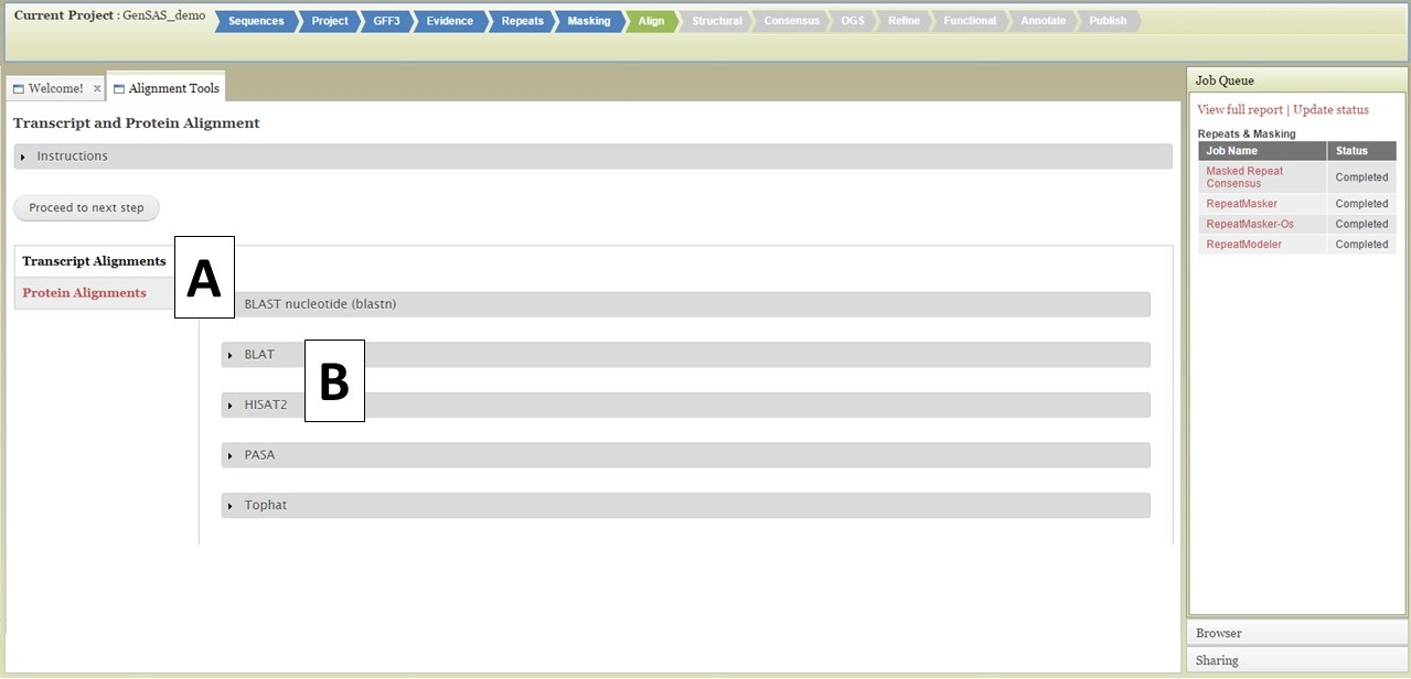
Figure 26. Align Tab in GenSAS.
For nucleotide BLAST, BLAT and PASA, there are global data files available to use. GenSAS provides the mRNA NCBI RefSeq datasets for all the major RefSeq categories (Fig. 27B). Any transcript and EST evidence files that you uploaded will also be available for use with these tools. For PASA, you will also have to select the "Vector FASTA file" in order for the tool to run (Fig. 28A). PASA checks sequences for vector contamination. As with the the repeat tools, please look at the results of these tools before using the data in downstream tools.
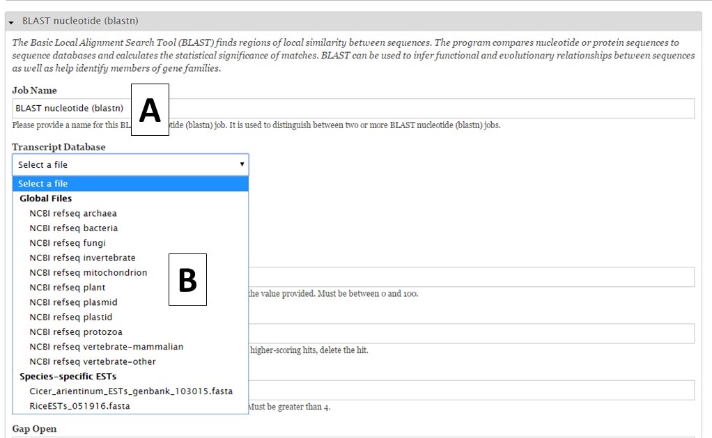
Figure 27. BLAST interface.
For RNA-seq reads, you can align them to the genome using HISAT2 or TopHat. This alignment can then be used to train Augustus during the "Structural" step. To align RNA-seq reads, either select the single read file or the paired read files (Fig. 28B) you uploaded during the Evidence step of GenSAS under the HISAT2 or TopHat job creation form. Please be aware that results from HISAT2 and TopHat job take awhile to load in JBrowse once the job has completed.
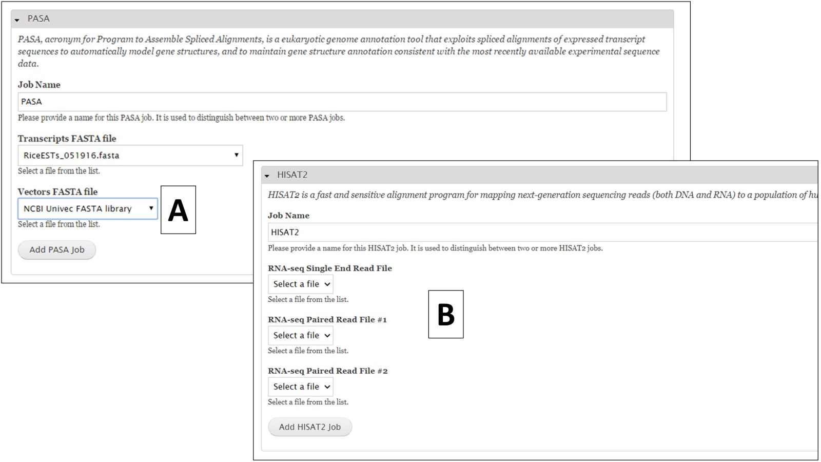
Figure 28. PASA and HISAT2 interfaces.
To set up a protein BLAST of DIAMOND job, click on "Protein Alignments" and then the tool name to access the job creation interface (Fig. 29A). During this phase of GenSAS, we only provide access to the RefSeq, SwissProt, and TrEMBL global databases for DIAMOND alignments becuase DIAMOND runs much quicker than BLAST. Under the "Functional" step of GenSAS, you will be able to run protein BLAST with these global databases since aligning gene models with these databases is less computationally intensive. Under the "Align" step, we do allow you to perform protein BLAST with species-specific evidence (Fig. 29B) that you have loaded into GenSAS during the "Evidence" step.
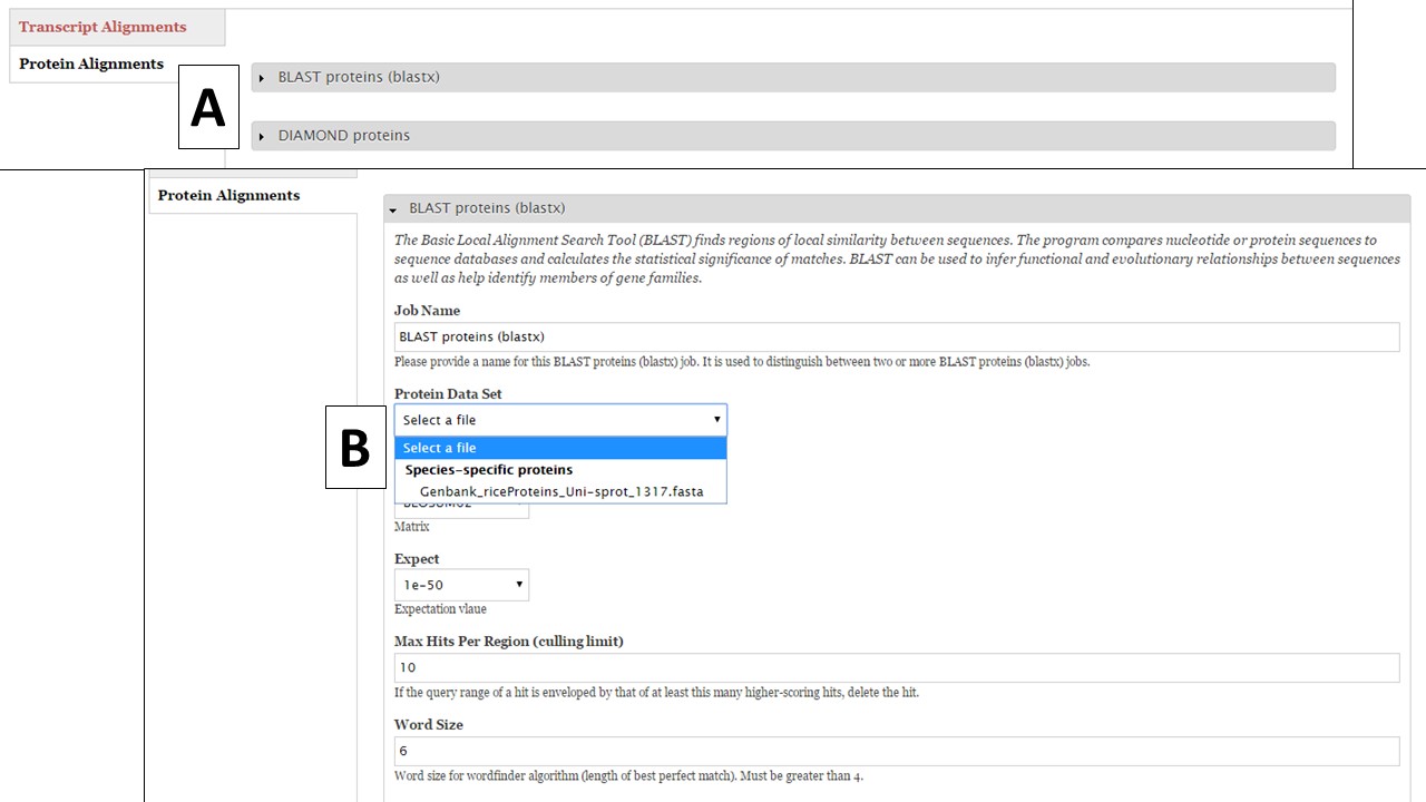
Figure 29. Protein BLAST under Align step.
Once you are done with setting up alignment tool jobs, click "Proceed to the next step" near the top of the tab to move to the "Structural" annotation step of GenSAS.
Structural Tab
The Structural step of GenSAS is where the gene prediction and other sturtural feature tools are run. For eukaryotes, the tools are described below. For prokaryotes, GeneMarkS, Glimmer3, RNAmmer, Getorf, and tRNAscan are available at this step. Please see below for examples of setting up jobs, the interfaces are very similar for the prokaryote-only tools. For detailed information on each tool, please use the links on the "Available Tools" table on the GenSAS homepage. There are two main types of tools available in this step: "Gene Prediction" and "Other Features" tools (Fig. 30A). Under the "Gene Prediction" section (Fig. 30B), there are six options and the settings for each tool are viewed by clicking on the tool name. As with the other GenSAS tools, you can run each tool multiple times with different settings as long as each job has an unique name.
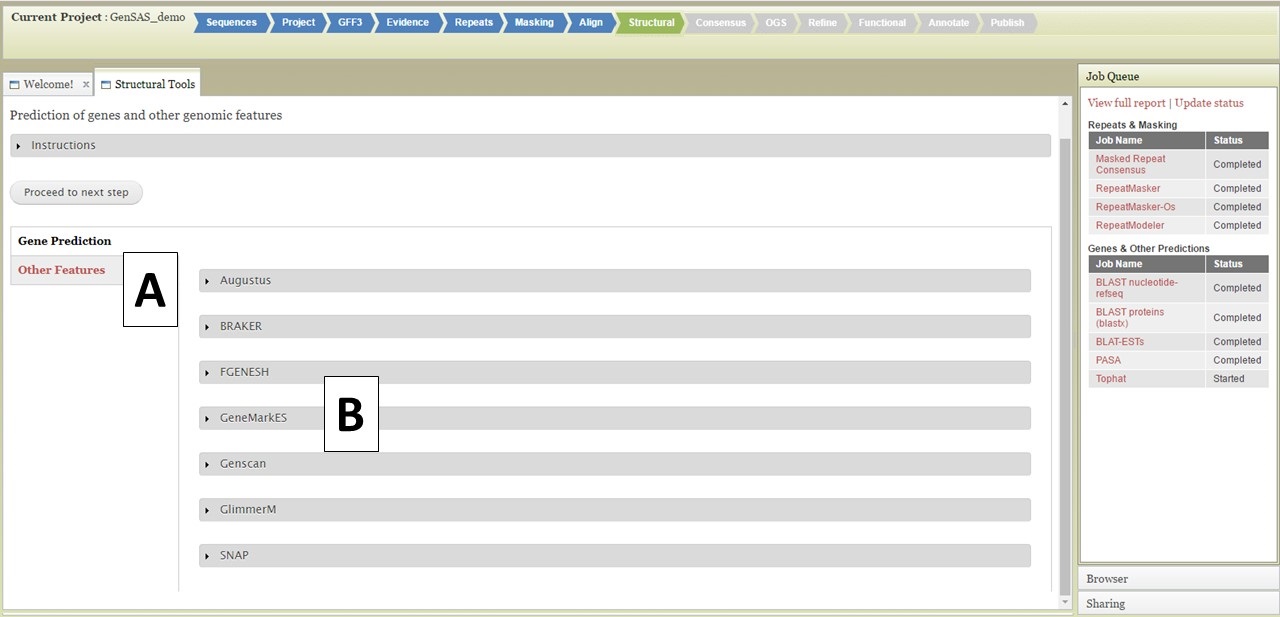
Figure 30. Structural step of GenSAS.
The first tool is Augustus, and this tool can be run with pre-trained datasets or you can train the tool for your organism using evidence you provide. If you would like to run Augustus with one of the provided organism settings,choose the species from the drop down menu (Fig. 31A), use or adjust the other settings, and then click on "Add Augustus Job" (Fig. 31B). If you would like to train Augustus, you can open the "Options for training Augustus" section (Fig. 31C). Under the training parameters section for Augustus (Fig. 31D), there are four data types. The selections for each type will depend on the evidence that has been uploaded to GenSAS and/or tools that have already been run. BRAKER requires a BAM file to run (Fig. 31E).
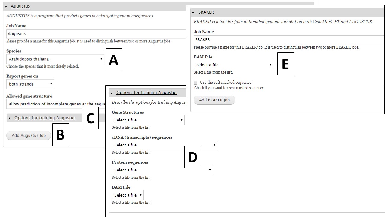
Figure 31. Augustus and BRAKER settings in GenSAS.
To train Augustus, one of data selections/combinations from Table 2 is required to set-up a training job. The data should be specific to the organism being annotated and can be uploaded under the "Evidence" step of GenSAS. The BAM file section will show the results from aligning uploaded RNA-seq reads to the genome with TopHat (from "Align" step). Once the appropriate data selections are made, click on the "Add Augustus Job" button to add a training job to the job queue.
| Training Option | Required Data Files to Select |
|---|---|
| Genes and Transcripts | "Genes Structures" (Genbank file) and "cDNA sequences" (FASTA file) |
| Proteins only | "Protein sequences" (FASTA file) |
| Proteins and Transcripts | "Protein sequences" (FASTA file) and "cDNA sequences" (FASTA file) |
| RNA-seq reads | Select the TopHat or HISAT job results or uploaded file under "BAM File" |
Table 2. Data type combinations needed to train Augustus.
If you are working on a non-model organism, and do not have species-specific evidence, GeneMark is a self-training gene prediction tool that might work well for your organism (Fig. 32A). In GenSAS, there is also an interface for FGENESH (Fig. 32B). Due to licensing restrictions, GenSAS cannot run this tool, but you can import the results from the tool and GenSAS will parse the data and make it available to use in downstream steps. GenSAS also has Genscan (Fig. 33A), GlimmerM (Fig. 33B), and SNAP (Fig. 33C). Genscan can only process DNA pieces shorter than 8 Mbp. If your assembly has scaffolds or contigs larger than 8 Mbp, Genscan will not return any results.
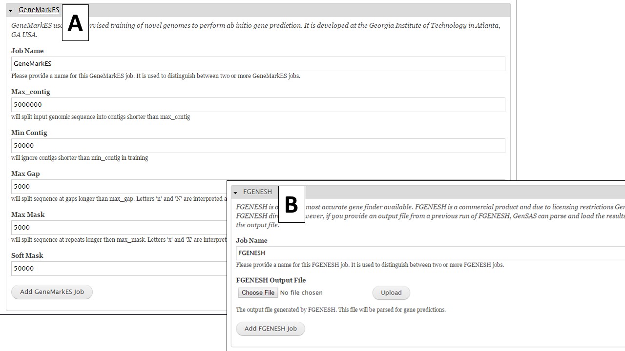
Figure 32. GeneMark and FGENESH interfaces.
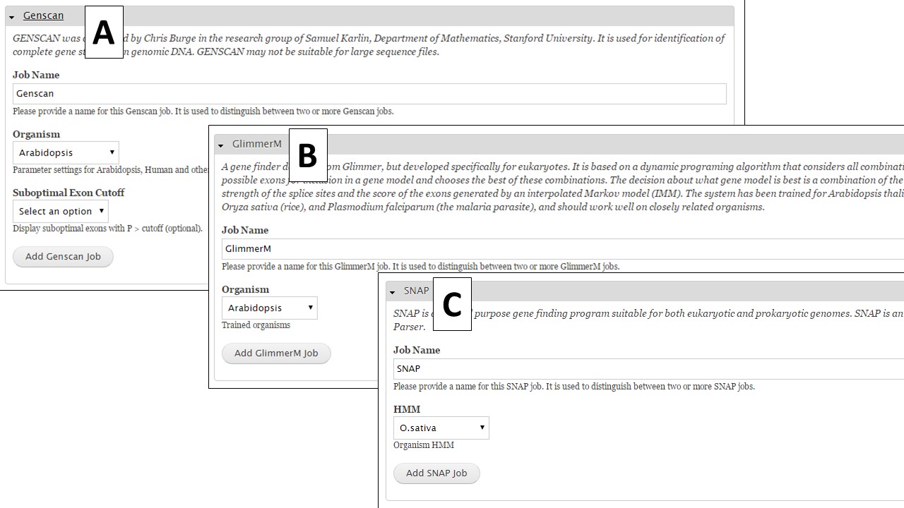
Figure 33. Genscan, Glimmer and SNAP interfaces.
Under the "Other Features" section (Fig. 34), there are four tools that identify other structural features. To identify tRNA and rRNA sequences, use tRNAscan-SE (Fig. 35A) and RNAmmer (Fig. 35B), respectively. Getorf is a tool to identify open reading frames (Fig. 35C). The SSRs tool (Fig. 35D) locates simple sequence repeats (SSRs). Please note that many SSRs are masked by Repeatmasker and RepeatModeler, so if you want a complete list of SSRs from your DNA it is best to run this tool on unmasked sequences.
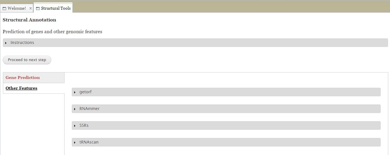
Figure 34. The Other Features section of Structural Tab.
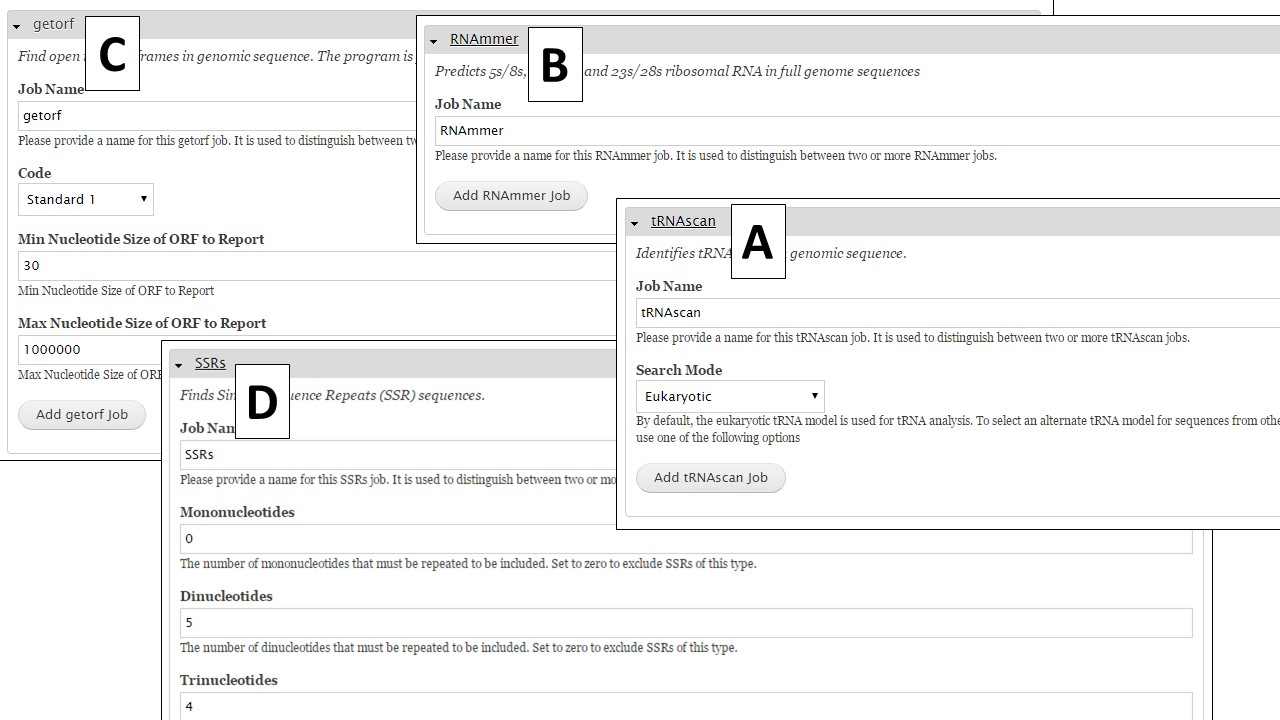
Figure 35. Interfaces for tRNAscan, RNAmmer, Getorf, and SSR tool.
You will be able to track the progress of all structural tool jobs via the Job Queue on the right of the GenSAS interface. As the jobs complete, the data can be viewed in JBrowse/Apollo. If you have JBrowse open when a job completes, you will have to reload JBrowse to view the new data (Please see Apollo and JBrowse section for more info). It is very important to look at the results from each tool and to determine if the data makes sense for your organism before using the results in downstream steps. Once you have completed running jobs under the "Structural" step and looked at the results, click on the "Proceed to next step" button to move on to the "OGS" step.
OGS Tab
In the "OGS" step, you will choose the set of gene models that will be designated the Official Gene Set (OGS). After manual curation, GenSAS will merge any user-created manual curations from Apollo into the OGS and produce the final annotation files at the "Publish" step. To assist with OGS selection, the option to run BUSCO on the candidate OGS tracks is available (Fig. 38A). To run BUSCO, check the box in the "BUSCO Job" column of the table (Fig. 38B), and then select the BUSCO dataset and click "Perform the action." Once the BUSCO jobs have completed, the results appear on the table and more detailed results files can be accessed by clicking on "completed" in the "BUSCO Job" column of the table.
You can choose to use the data from a single tool, genes consensus job, or previously imported annotation as the OGS. Just click on the circle next to the dataset you want to designate as the OGS (Fig. 8D) and then click on the "Use selected job for OGS" button. Once an OGS is selected or created, the "Refine" step becomes available for use. If you later change your mind about what to use for the OGS, just open the OGS tab and click on the "Change the OGS" button. However, to change the OGS there cannot be any "Refine" or "Functional" jobs that have been run or are running with the current OGS. If there are such jobs present, delete those jobs and GenSAS will allow for the OGS to be changed.

Figure 38. Selecting a dataset to use as the OGS.
Refine Tab
Under the "Refine" step, you have the option of running PASA again to refine the gene models of the official gene set (OGS). The OGS will be listed on the interface (Fig. 39A), and you can either run the refinement by setting up the PASA job below (Fig. 39B), or you can skip this step by clicking on the "Proceed to the next step" button. If you do set-up a PASA refinement job, a summary screen appears after the job is submitted (Fig. 39C). The gene model refinement step works best with species-specific transcript data. Once the PASA refinement job has completed, the "Functional" step will become available. The Refine tab is only available to eukaryotic organisms.
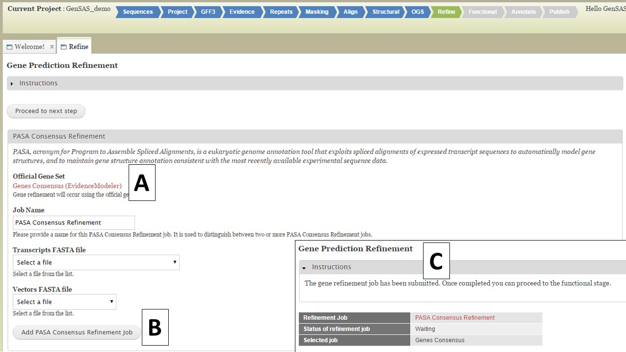
Figure 39. Refine step of GenSAS.
Functional Tab
Under the "Functional" step of GenSAS, you can run tools that will help assign a function to the proteins encoded by the predicted gene models. There are five tools available (Fig. 40): protein BLAST, DIAMOND, InterProScan, Pfam, SignalP, and TargetP. TargetP is only available to eukaryotes. For the "Functional" step, you will only be able to run the tools on the OGS. If you have refined the OGS, the gene set from the "Refine" step will be used. You can run each tool mulitple times with different datasets and/or settings, as long as each job has an unique name.
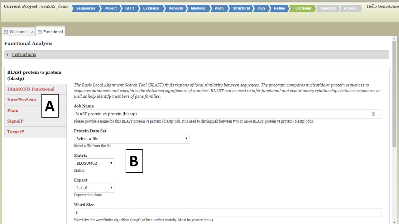
Figure 40. Functional step interface.
For protein BLAST, several global protein datasets are available along with user uploaded protein data. The RefSeq protein sets for the NCBI organism groups and the SwissProt and TrEMBL datasets are available to use. We recommend using SwissProt since this is a curated protein database and only contains proteins that have been functionally curated, and as a result, will provide more reliable functional annotations. InterProScan looks for protein functional domains while SignalP and TargetP identify signal peptides for cleavage sites and subcellular localization, respectively. The Pfam tool will identify functional domains and protein families. Functional jobs will appear in the Job Queue. To view the functional tool results, click on the job name in the Job Queue (Fig. 41A). The job details tab will open (Fig. 41B) and there will be a table of all the gene models on the lower right (Fig. 41C). There will not be any summary numbers in the "Predicted Annotations" and "Annotations Per Sequence" tables for any of the functional annotation tools. To view all the functional results associated with the gene model, click on the gene ID (Fig. 41C) and another tab will open that contains all the functional annotation results for that gene model (Fig. 41D). If there was a result for any of the functional tools for that gene model, the results will appear on this tab and you can view the results from each tool by clicking on the tool name on the left (Fig. 41D).
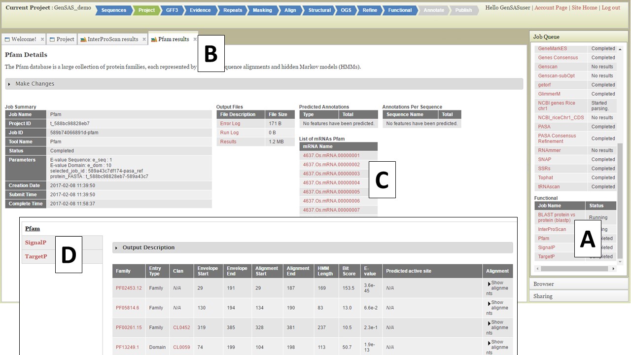
Figure 41. Gene Model functional results table.
The gene model functional results tab can also be accessed through JBrowse. In JBrowse, right click on the gene model and a menu appears. Then select the "View putative annotations" option (Fig. 42A) and the tab with the functional annotation information will appear (Fig. 42B).
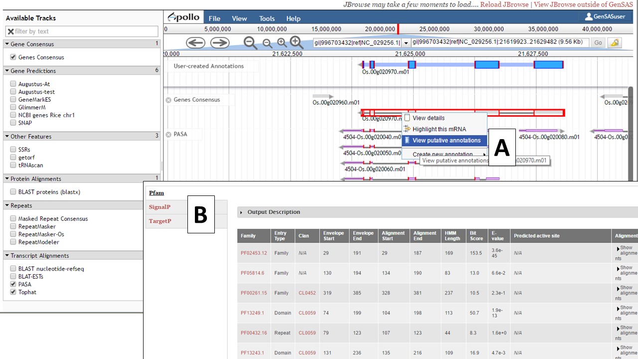
Figure 42. Accessing gene model functional annotation results in JBrowse.
Once you have finished setting up functional annotation jobs, click on the "Proceed to next step" button to move to the "Annotate" step.
Sharing Projects
You can share your GenSAS project once a job has completed in the Job Queue, and you can open Apollo/JBrowse. To share a project, open the "Sharing" section of the right-side accordian menu (Fig. 43A) and click on "Share this Project." The "Project Sharing" tab will then open and you can open the "Share this Project" interface (Fig. 43B). You will need to know the GenSAS user name for the person you want to share the project with. Type the GenSAS user name into the box, and then select either read-only access or full access and click "Add User." Users who have read-only access will only be able to view the data, users with full access will be able to run jobs and perform manual curations under the "Annotate" step. The list of users the project is shared with, can be viewed under the "Sharing" section of the Job Queue (Fig. 43A) or on the "Project Sharing" tab (Fig. 43C). If you want to change the sharing permissions, or stop sharing your project, just open the "Project Sharing" tab and go to the user name on the table (Fig. 43C). Click to change the sharing level under the "Permission" column of the table, or click on the "Remove Sharing" link under the "Action" column.
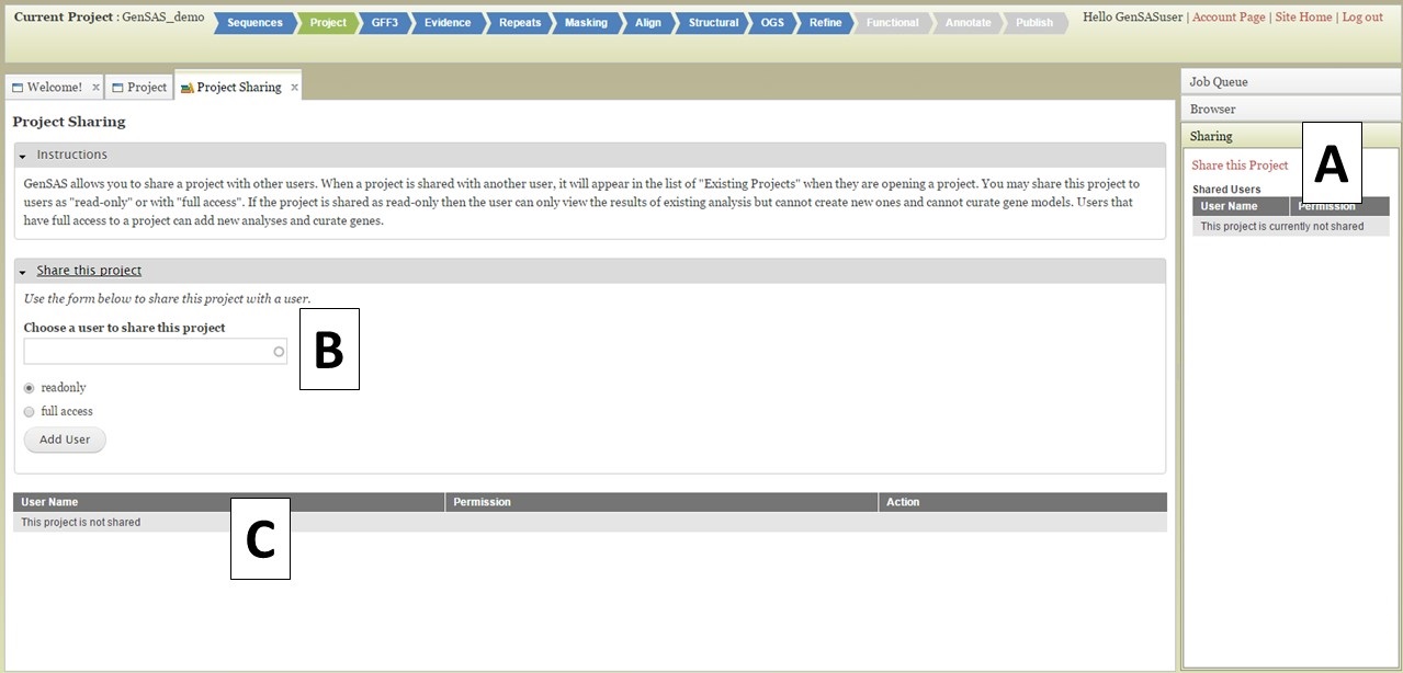
Figure 43. Project Sharing tab in GenSAS.
Annotate Tab
Under the "Annotate" step you have the option of performing manual curation. While manual curation is not required, we suggest at least looking at several gene models and the output from the tools along with provided evidence to see if the gene models are most likely accurate. The manual curation function in GenSAS is performed using an integrated Apollo instance. Apollo not only provides manual curation functionality, but also tracks all changes made and which user made them on the "Apollo" tab, which is useful for collaborative annotation projects. To learn how to share your GenSAS project, please see the "Sharing Projects" section of the User's Guide.
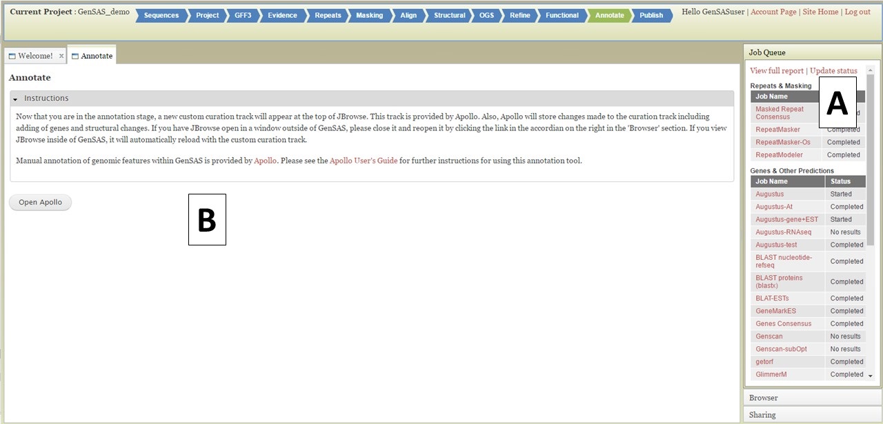
Figure 44. Annotate tab in GenSAS.
Under the "Annotate" tab, you will see a "Open Apollo" button (Fig. 44B). You can either open Apollo using that button, or open Apollo through the "Browser" section of the Job Queue (Fig. 44A). Please see the "Apollo and JBrowse" section on details on how to open Apollo/JBrowse. In the "Apollo" tab, there is a JBrowse interface on the left and you will now see a "User-created Annotations" track at the top (Fig. 45A). This is where any manual annotation changes will be entered. The changes made to the "User-created Annotations" track are logged on the Apollo interface on the right, under the "Annotations" tab (Fig. 45B). To control which data tracks are visible in JBrowse, click on the "Tracks" tab in the Apollo interface (Fig. 46A). Expandable sections appear for each data track type. Expand the section and toggle the tracks on and off. If you would like to use the normal JBrowse Track Selector, you can also toggle that on and off in the Apollo interface (Fig. 46B).
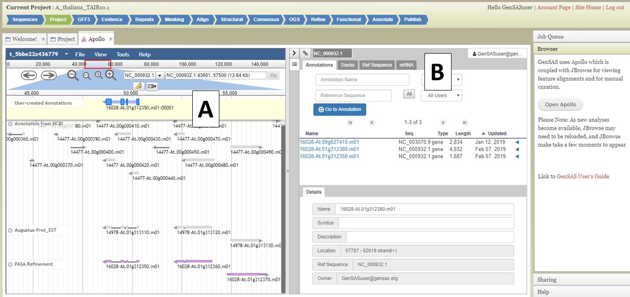
Figure 45. User-created Annotations track in JBrowse.
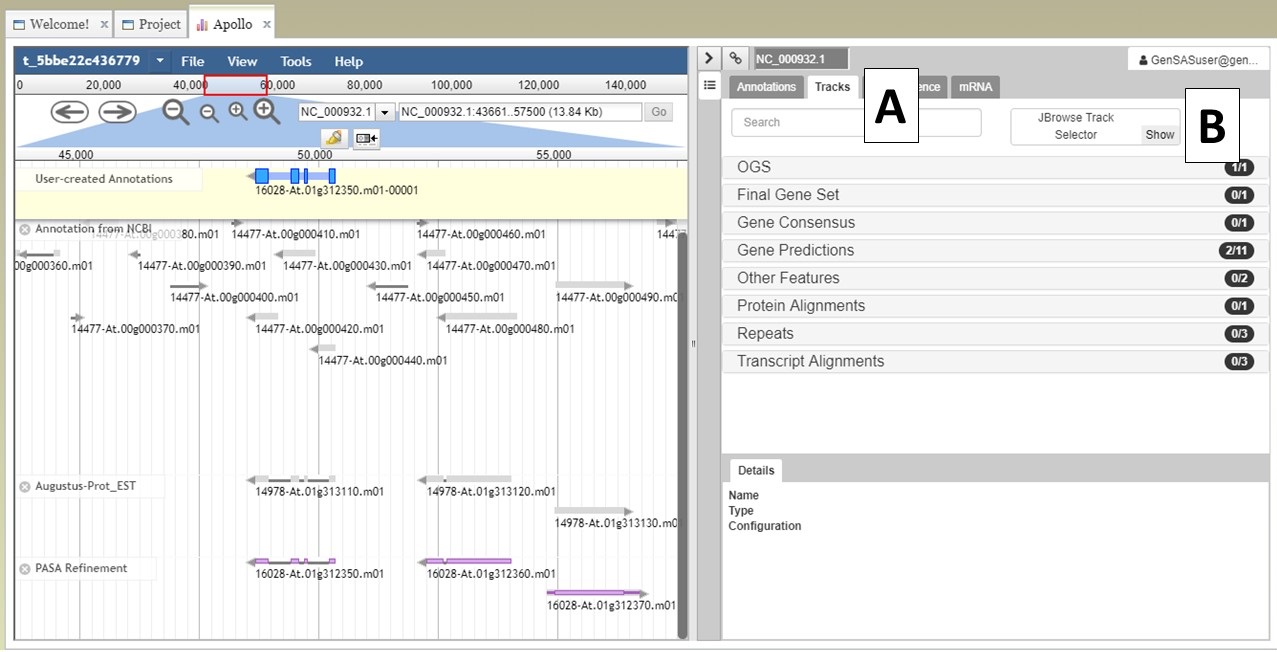
Figure 46. Turning tracks on and off in JBrowse window.
For detailed instructions on Apollo, and some information on manual curation, we recommend the Apollo User's Guide. Another good resource is "Annotation for Amateurs" which has tutorials on annotation. Per the Apollo manual, the major steps of manual curation are:
- Locate a region of the chromosome that you want to annotate in the JBrowse tab and look for gene models that might need manual curation.
- Look at the job and evidence tracks and decide if there is a likely gene model to use as a starting point.
- Drag the putative gene model to the "User-created Annotations" track to use as the initial gene model.
- Edit the gene model structure (UTRs, intron/exon junctions, start/stop codons) if necessary.
- Check the edited gene model against existing homologs by exporting the sequence and searching a protein database.
- Assign functional assignments using the Gene Ontology (GO) database and add the information to the feature notes.
Not all gene models will need editing, but some gene models will benefit from manual curation. In the GenSAS User's Guide we will only cover the basics of using Apollo and provide some examples of manual curation (see example below). To move a gene model to the "User-created Annotations" track, double click on the model until it is highlighted with red borders (Fig. 47A) and then click and drag the model to the "User-created Annotations" track (Fig. 47B). Also note that when a gene model is selected, common intron/exon junctions across all datasets are also indicated with red borders (Fig. 47C).
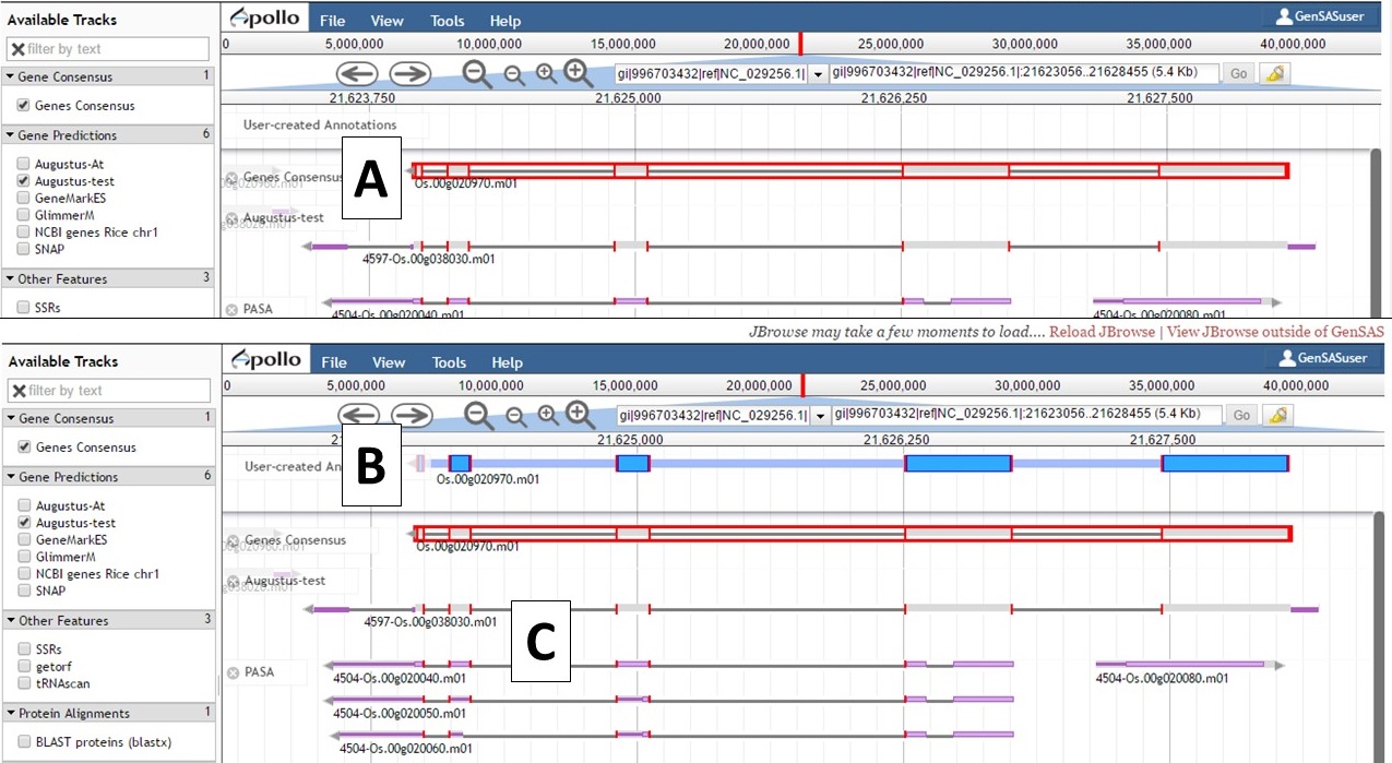
Figure 47. Dragging gene model to User-created Annotations track.
Once the gene model of interest is in the curation track, you can zoom in to the base level quickly by right-clicking on the model and selecting the "Zoom to base level" option (Fig. 48). This is useful for looking at intron/exon junctions and start/stop codons. You can also download the nucleotide or protein sequence of the gene model by right-clicking on the gene model and selecting the "Get sequence" option (Fig. 49). This is useful for getting the protein sequence for searches against a protein database during the manual curation process.
.jpg)
Figure 48. Zooming to base level of gene model.
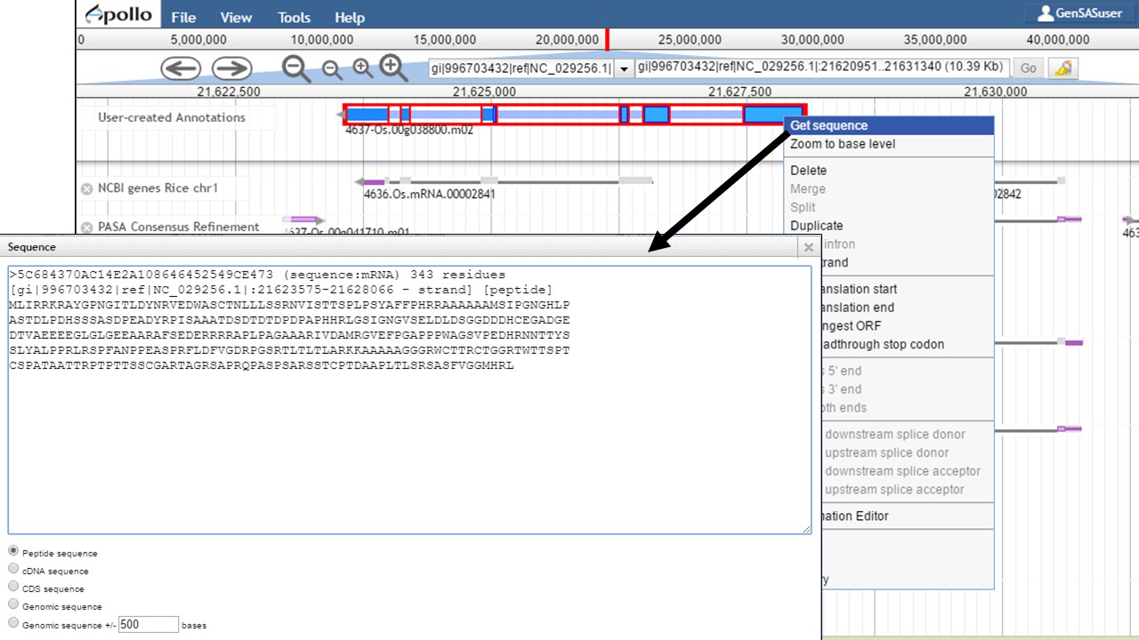
Figure 49. Obtaining sequence of gene model.
Here is an example of a manual curation of a gene model in chromosome 1 of rice. In Figure 50, you will see the JBrowse window at the "Annotate" step. The data tracks are marked to help describe the data that will be used:
- "NCBI annotation" is the imported GFF3 data of the annotation that is available in NCBI for the sequence (chromosome 1 of rice).
- "Refined Consensus" is a genes consensus that was created in GenSAS at the "OGS" step and was then refined with rice ESTs (from NCBI, uploaded by user) during the "Refine" step.
- "Augustus-RNA-seq trained" is the results of a trained Augustus job using the BAM file from the TopHat alignment of RNA-seq reads to the sequence being annotated.
- "PASA, rice ESTs" is a PASA job from the "Align" step that used rice ESTs that were uploaded by the user.
- "TopHat, rice RNA-seq" shows the results of the TopHat alignment of the user-uploaded RNA-seq reads to the sequence being annotated.
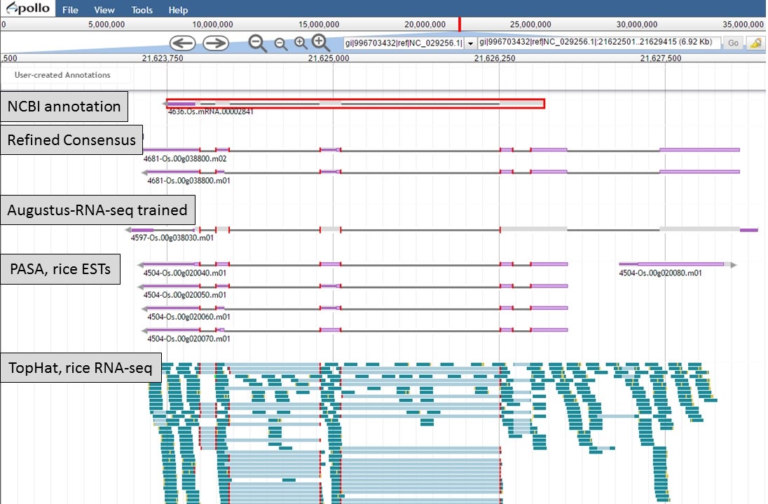
Figure 50. Manual curation example. See track descriptions above figure in text.
You can see that when the NCBI gene model is selected (Fig. 50), that the common intron/exon junctions are marked across all datasets in JBrowse. Also notice that there are differences between the annotation from NCBI and the alignments and gene predictions job results based on transcript evidence. This looks like a good candidate for manual curation. For this example, let's move the gene models we want to compare to the "User-created Annotations" track. Based on the RNA-seq data, let's look at a gene model from the "Refined Consensus" track (Fig. 51A), "PASA, rice ESTs" track (Fig. 51B), and the "NCBI annotation" track (Fig. 51C). Figure 51 is marked to show which gene model in the "User-created Annotations" track corresponds to which gene model in the evidence tracks.
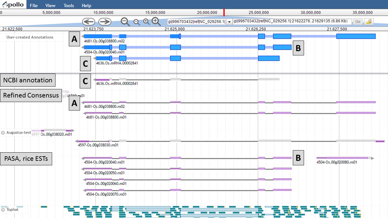
Figure 51. Three gene-models moved to User-created Annotations track.
Since there is RNA-seq evidence for this project, let's compare each of these gene models to the RNA-seq data (you can use EST evidence alignments if you don't have RNA-seq data). In Figure 52, the gene models from the "NCBI annotation" and "PASA, rice ESTs" are selected and show that most of the intron/exon junctions in these gene models are supported by the evidence in the other tracks (see red marks at junctions within black boxes). When the gene model from the "Refined Consensus" is selected (Fig. 53), most of the intron/exon junctions are not supported by the evidence except for a few (see inside black box).
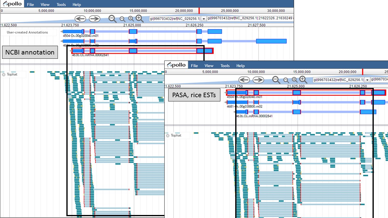
Figure 52. Intron/exon junctions in NCBI and PASA based gene models are supported by other data.
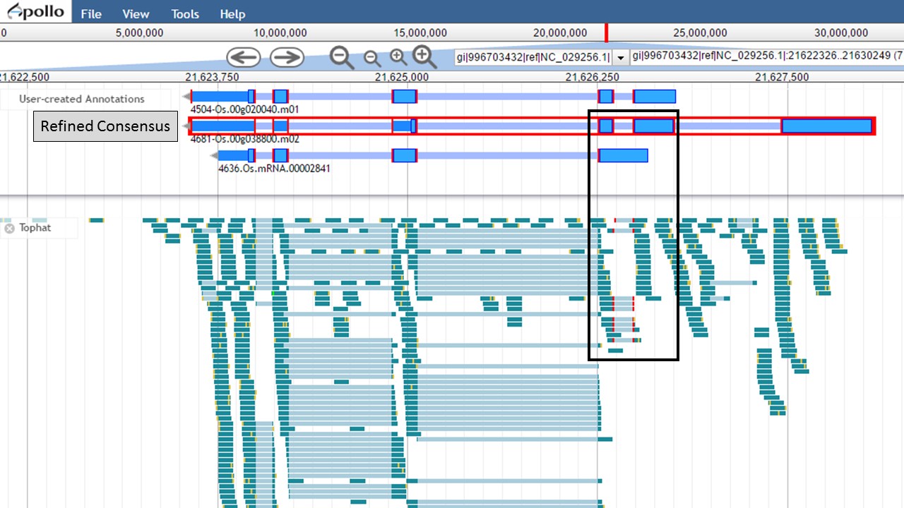
Figure 53. Few intron/exon junctions in Refined Consensus gene model are supported by other data.
Since the "Refined Consensus" gene model is not very well supported by transcript data, let's delete it from the "User-created Annotations" track. Select the gene model by double-clicking on it, then right-click with the mouse and select the "Delete" option (Fig. 54).
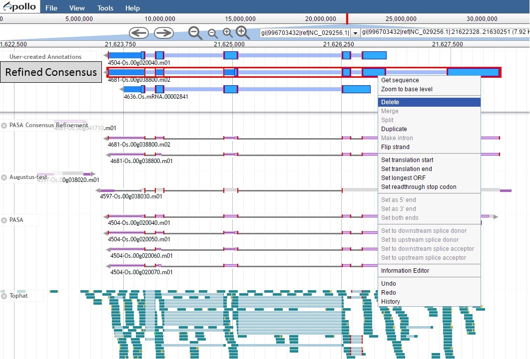
Figure 54. Deleting a track from the User-created Annotations track.
Now there are two gene models left, the "NCBI annotation" and the "PASA, rice ESTs" models (Fig. 55). The two gene models have different start positions and both lack 5' UTRs.
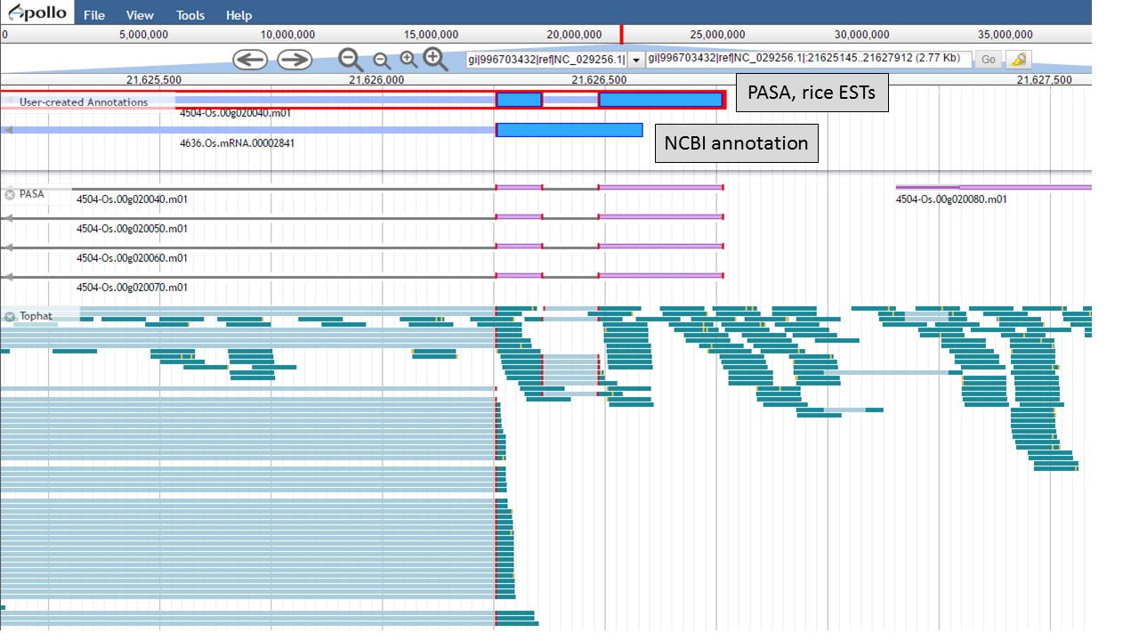
Figure 55. Two remaing gene models, with different start positions.
Let's look at the start codon for each model. When we zoom in to the base level (see Fig. 48 above for directions), we see that the start codon for the NCBI annotation is "ATG" and the start codon for the PASA gene model is "AAG" (Fig. 56). Since the PASA gene model is based on alignments with ESTs, the gene model structure was based on matches with EST evidence. This means that the location of the start on the PASA gene model is more likely the start of the 5' UTR.
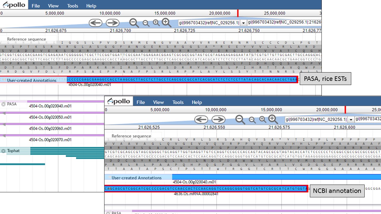
Figure 56. Start codon sequences on both gene models.
To set the translation start on the "PASA, rice ESTs" gene model, use the "NCBI annotation" start codon location as a guide to find the start codon. Once the start codon of "ATG" is located on the "PASA, rice ESTs" sequence, place the cursor at the beginning of the codon, right-click and select the "Set translation start" option (Fig. 57).
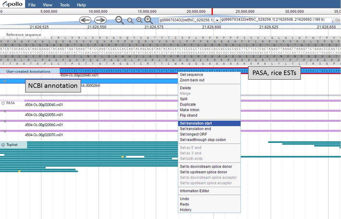
Figure 57. Setting translation start on "PASA, rice ESTs" gene model.
Both gene models now have the same start codon, but the "PASA, rice ESTs" model also has the 5' UTR region (Fig. 58).
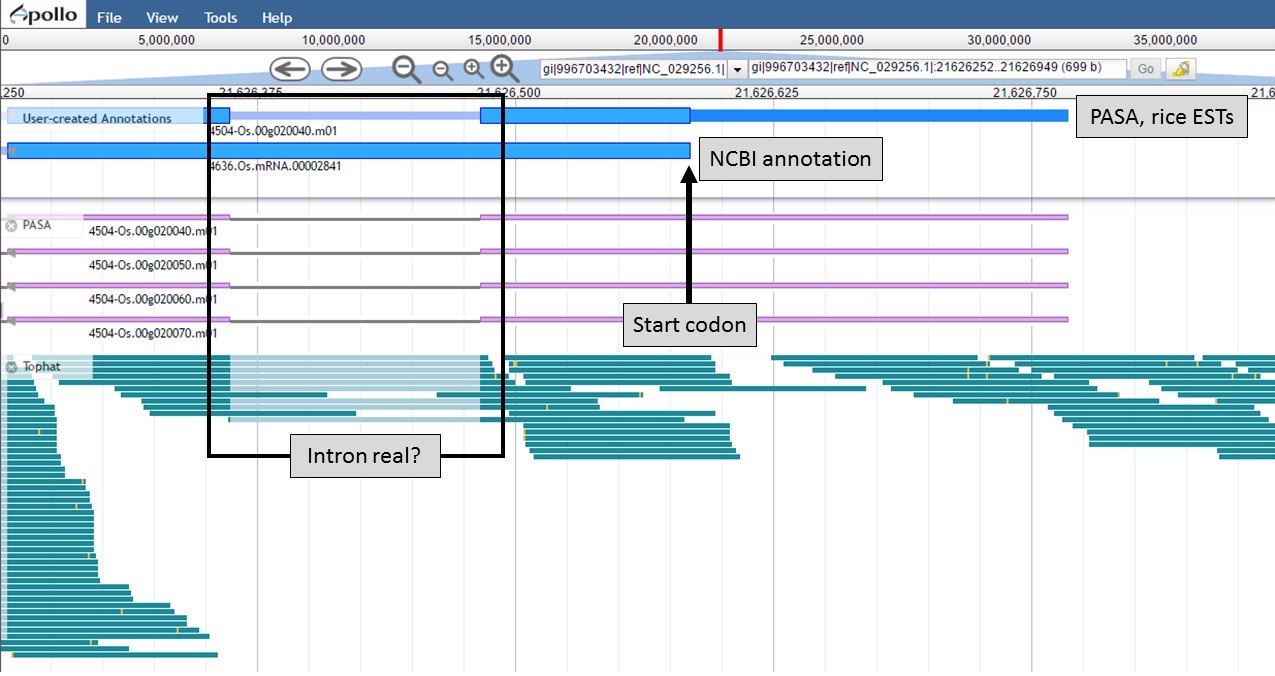
Figure 58. New 5' end of gene models and closer look at intron region.
At the 3' end of the gene model, the stop codons are in the same location, but the transcript evidence is supporting a longer 3' UTR region in the "PASA, rice ESTs" model (Fig. 59). Based on the evidence, the 3' UTR of the "PASA, rice ESTs" is probably more accurate.
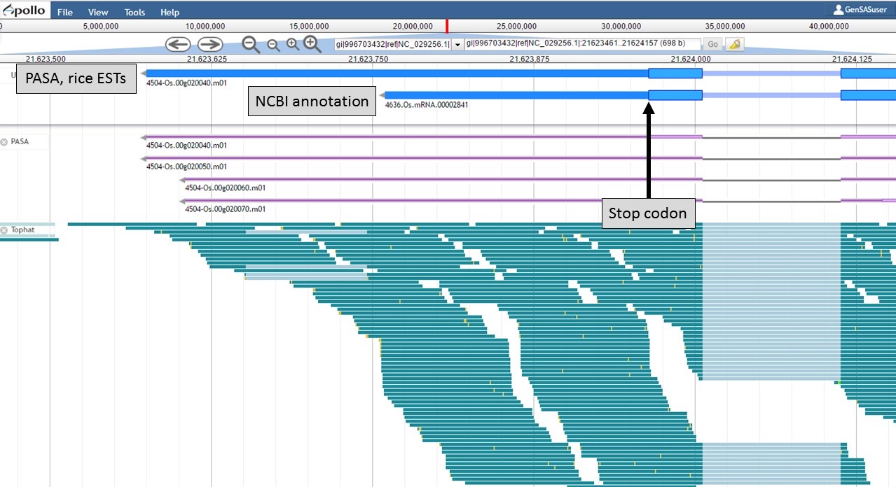
Figure 59. 3' end of gene models.
Now that the ends of the gene models have been examined, we need to determine if the first intron in the "PASA, rice ESTs" gene model is real or not. In Figure 58, a box around the intron area shows that there is EST and RNA-seq evidence support for the intron in the "PASA, rice ESTs" model. Let's look closer at the proteins coded by these gene models. Using the "Get sequence" function for each gene model (see Fig. 49 above for directions), we see that each gene model produces a different length protein (Fig. 60). The "NCBI annotation" gene model only encodes for a protein of 60 amino acids long while the "PASA, rice ESTs" gene model produces a protein of 176 amino acids. If we look closer at the "NCBI annotation" gene model, there is a stop codon in the gene model after 60 amino acids. The stop codon in the "NCBI annotation" model also sits within the intron of the "PASA, rice ESTs" gene model that is missing from the "NCBI annotation" (Fig. 58). If you look at the protein sequence alignment in Figure 60, the amino acids that are in bold correspond the first exon of the "PASA, rice ESTs" gene model. The exon-intron splice site sequences can also be examined. The common eukaryotic splice junction has a structure of 5'-exon]GT/AG[exon-3'. If the splice site is non-canonical, Apollo marks it with a orange exclamation mark so the annotator will take a closer look.
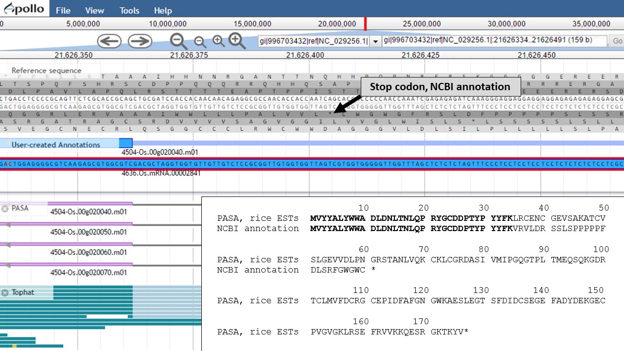
Figure 60. Proteins from each gene model and the location of the stop codon in the NCBI annotation model.
But which protein is more likely? Let's use NCBI protein BLAST to see if there are any related proteins. You can also use SmartBLAST which compares the closest protein matches graphically (Fig. 61). The protein encoded by the "PASA, rice ESTs" model has a DUF866 domain and is similar to other proteins of unknown function. The protein from the "NCBI annotation" is a truncated version of the same unknown protein. This indicates that the "PASA, rice ESTs" gene model that we edited is not only supported by the EST and RNA-seq evidence, but also by protein similarity.
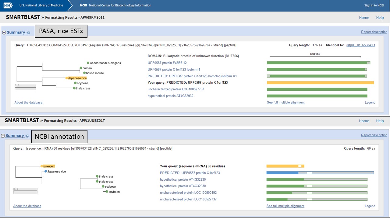
Figure 61. SmartBLAST results of proteins derived from gene models.
Since the "PASA, rice ESTs" gene model is supported by the evidence, the "NCBI annotation" gene model needs to be deleted from the "User-created annotations" track (see Fig. 54 above for instructions). We can now focus on the final edited gene model and can add information to the feature information. To do this, double-click the gene model to select it and then right-click and choose the "Information Editor" option (Fig. 62).
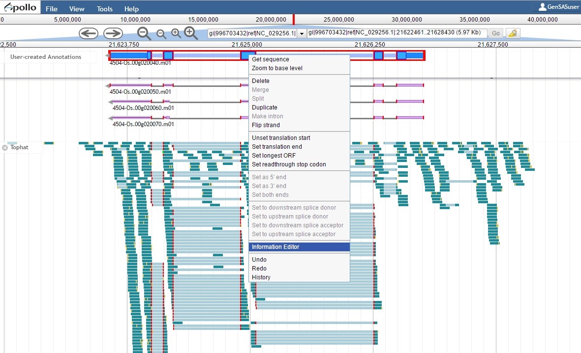
Figure 62. Opening the Information Editor window.
A pop-up window opens and has fields for the gene and mRNA annotations (Fig. 63). You can enter information in the boxes by clicking "Add" and then entering info into the field that appears.
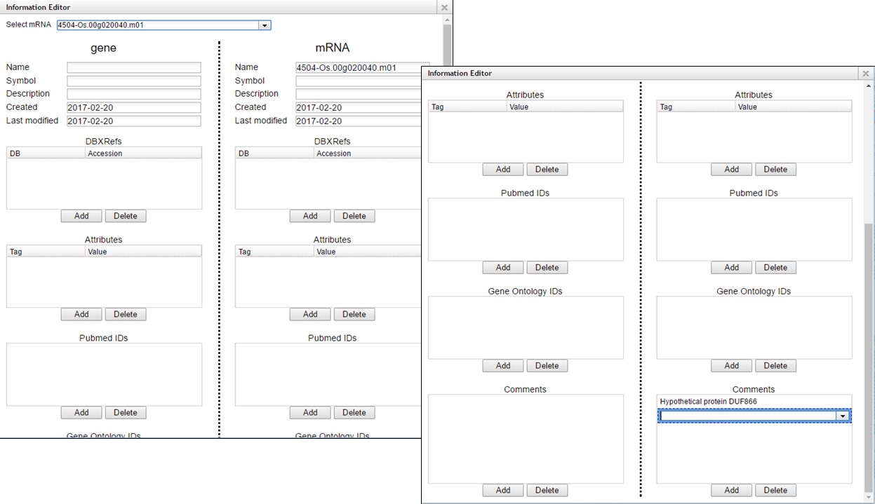
Figure 63. Information Editor window fields.
Once you have completed manual curation, you can prepare the final files by going to the "Publish" step.
Publish Tab
On the "Publish" step, you will generate the files needed for publication or use with downsteam tools. GenSAS outputs the data in GFF3 and FASTA file formats. Any manual curation changes made in the "User-created Annotations" track in JBrowse/Apollo will be merged into the OGS at this step. GenSAS will also add assembly and annotation version numbers to the output files. You can choose which data is exported during this process, but GenSAS automatically selects the minimum files needed (Fig. 64). GenSAS will automatically publish the OGS, the associated gene models and sequences, and the masked repeat consensus. You can select to publish the results from the repeat, gene model prediction, alignment, other structural feature, and functional tools.
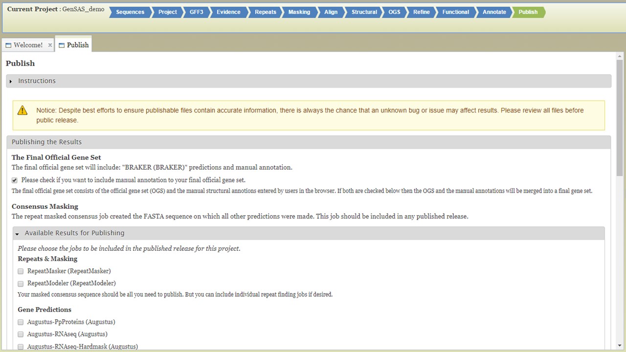
Figure 64. GenSAS "Publish" tab.
Once you have selected the datasets that you want output, click on the "Publish" button and an "Annotations" job will appear in the job queue. If you come back to GenSAS and make changes, you can generate version 2 of the annotation, with the new changes, by running another job under the "Publish" tab. Once the publish job is completed, access and download the files by clicking on the annotation job name in the job queue. Please note that GenSAS will remove proteins under 30 amino acids in length in the final published files. This will open the job summary tab (Fig. 65). The job summary tab has many different sections. At the very top is a button to create a merged GFF3 file (see more below). Nest, is a job summary table which lists which jobs were included in the final files, which track was the OGS, and a link to download a Project Summary file (Fig. 65B) that contains all the settings from the tools used to create the OGS. Below the project summary, is the list of generated files that can be downloaded (Fig. 65C). You can then click on the file names to download the files to your computer. If you want to download all the files at once, click on the "Download all" button at the end of the list (Fig. 65D). At the very bottom of the page is the option to run BUSCO on the predicted proteins of the final annotation (Fig. 65E).
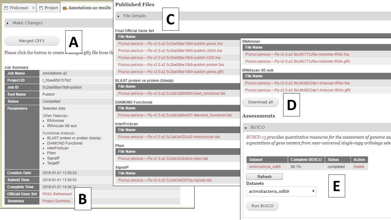
Figure 65. Annotation job results.
The option to create a merged GFF file (Fig. 65A) allows the user to add the repeats from RepeatMasker and Repeat Modeler and the rRNAs and tRNAs from RNAmmer and tRNAScan-SE into the GFF3 file of the OGS (FIg. 66A). The option to also add some of the functional annotation data into column 9 of the GFF3 is also present. After the file is generated, it can be downloaded by opening the "Merged GFF3" interface and clicking on the file name in the table at the very top of the page (Fig. 66B).
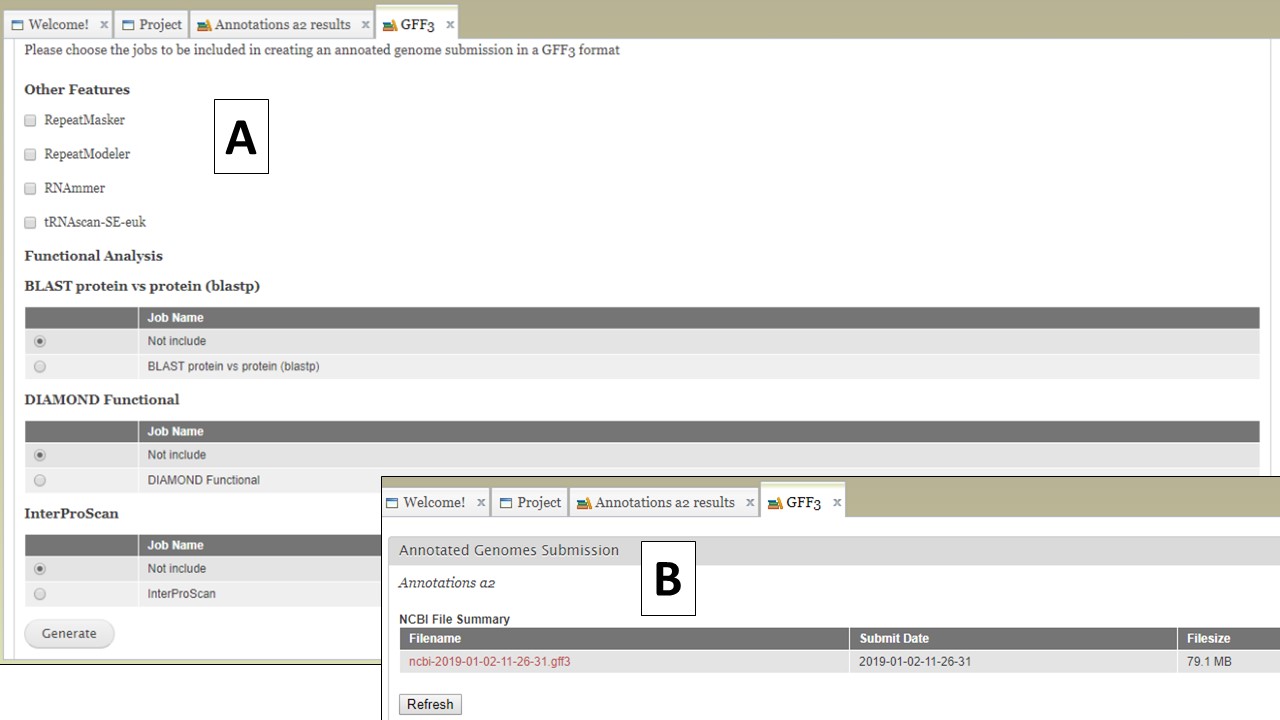
Figure 66. Creating a merged GFF3.
Editing Existing Jobs
If you open the job details tab by clicking on the job name in the job queue, you will see a "Make Changes" section that can be opened by clicking on it (Fig. 67A). You should not need to use this section, but occasionally there might be a need to. For most jobs, there are options to re-run and re-parse the job (Fig. 67B). Depending on when and why a job fails, these might be useful. Please note that if you have a job that fails (repeatedly), it is more likely a GenSAS bug or a problem with the input evidence files and we ask that you do not delete the failed job and contact us. If you want to delete a job, and the job results have not been used as input for another step (i.e. used to make a genes consensus), there will be a button to delete a job (Fig. 67C). Please be aware that any deleted jobs are not recoverable. If there is not an option to delete a job, it is because the results from the job have been used as input in a downstream tool. The downstream jobs that use the results have to be deleted first.
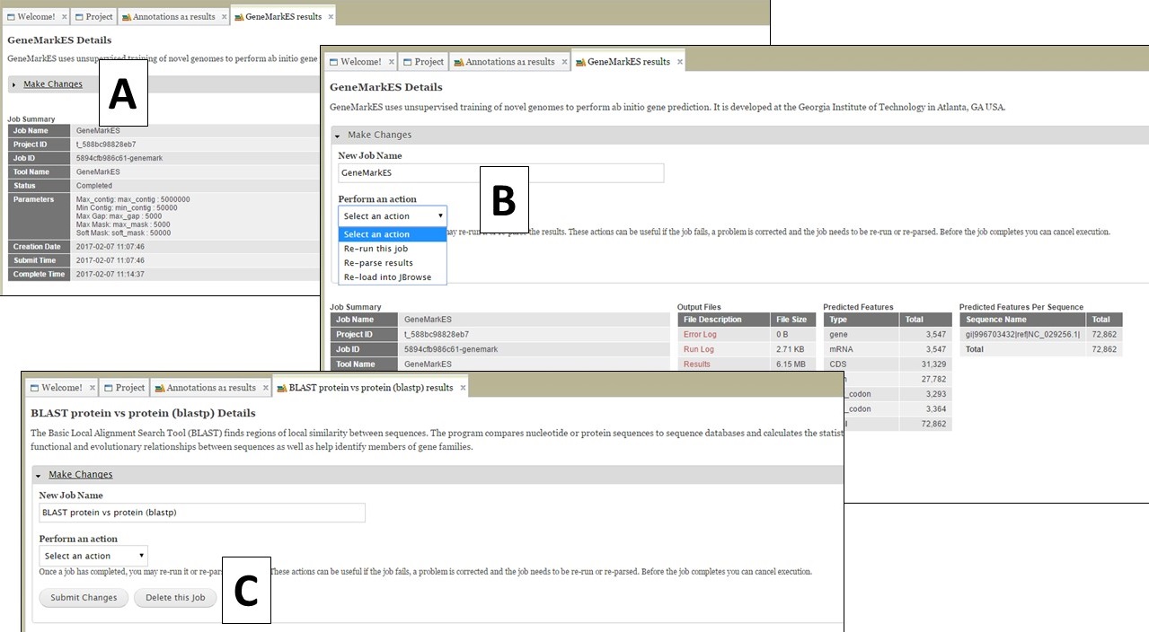
Figure 67. "Make changes" section on job results tabs.
Troubleshooting
Having problems with GenSAS? Please see the below troubleshooting table and if the problem persists after trying these fixes, please contact us.
| Problem | Solution |
|---|---|
| I cannot log into GenSAS | Please clear the cached images/files, cookies, and hosted app data from your internet browser's history |
| The request for a new password isn't working | Please clear the cached images/files, cookies, and hosted app data from your internet browser's history |
| JBrowse/Apollo will not load | Please clear the cached images/files, cookies, and hosted app data from your internet browser's history. You will have to log back into GenSAS and reopen your project. |
| The sequences I loaded are not available to select for a project | If you just uploaded a large sequence file immediately before project creation, please allow time for GenSAS to process the sequence file. Alternatively, your sequence file may have not passed the screening process. |
| GenSAS won't load a file because it already exists in GenSAS | We are working on fixing this, but in the meantime, please give the file you are trying to load a different name and upload it to GenSAS. |
| My large sequence or evidence files won't upload (>2 Gb) | Please contact us and let us know the file size(s) and the number of sequences in the file (for assemblies), and we will assist you. |
| My job is marked as "complete" in job queue, but I don't see it in JBrowse | For certain jobs, the job is marked complete in the Job Queue but is still being loaded into JBrowse. Your job is 100% complete and visible in JBrowse when you receive the email from GenSAS saying that the job is complete. |
| The GenSAS interface doesn't appear as in the manual | If you are using the Safari browser, GenSAS sometimes does not display correctly. We recommend using Chrome or FireFox. Also, if you have used the "zoom" function of your browser to zoom into the page, it may also cause the GenSAS interface to not appear correctly. Reset the page magnification to 100% and the problem should be resolved. |